3 Baseline Equivalence

In the quest to discern the true impact of an intervention, we must first establish a level playing field. The concept of baseline equivalence serves this purpose, ensuring that the groups under comparison are similar enough in key observed characteristics before the intervention takes place. Any discrepancies at baseline could muddy the waters, making it difficult to isolate the intervention’s effect from pre-existing differences.

Baseline equivalence is particularly crucial in scenarios where sample sizes are small or when we’re dealing with observational studies. Let’s say a company wants to evaluate a new algorithm designed to boost user engagement. If the group exposed to this new algorithm (the treatment group) already exhibited higher engagement levels than the control group prior to the experiment, any observed increase could simply be a continuation of their existing behavior, not necessarily a testament to the algorithm’s effectiveness.

3.1 Gauging Baseline Equivalence

To ascertain baseline equivalence, we turn to pre-intervention outcomes and other relevant observables. A common approach is to calculate the effect size, a standardized measure of the magnitude of an effect.

For continuous variables, Hedges’ g statistic is a popular choice (Hedges (1981)):

\[ g = \frac{\omega(y_t-y_c)}{\sqrt{\frac{(n_t - 1) s_t^2 + (n_c - 1) s_c^2}{n_t+n_c - 2}}} \] where

$y_t$ is the mean for the treatment group
$y_c$ is the mean for the comparison group
$n_t$ is the sample size for the treatment group
$n_c$ is the sample size for the comparison group
$s_t$ is the standard deviation for the treatment group
$s_c$ is the standard deviation for the comparison group
$\omega := 1 - \frac{3}{4(n_t+n_c)-9}$ is the small sample size correction.

For binary outcomes, Cox’s index comes into play (see Cox (1972)):

\[ d = \omega \left[ \ln\left(\frac{p_t}{1-p_t}\right) - \ln\left(\frac{p_c}{1-p_c}\right) \right] \] where:

$p_t$ is the the mean of the outcome in the intervention group
$p_c$ is the mean of the outcome in the comparison group
$\omega := 1 - \frac{3}{4(n_t+n_c)-9}$ is the small sample size correction.

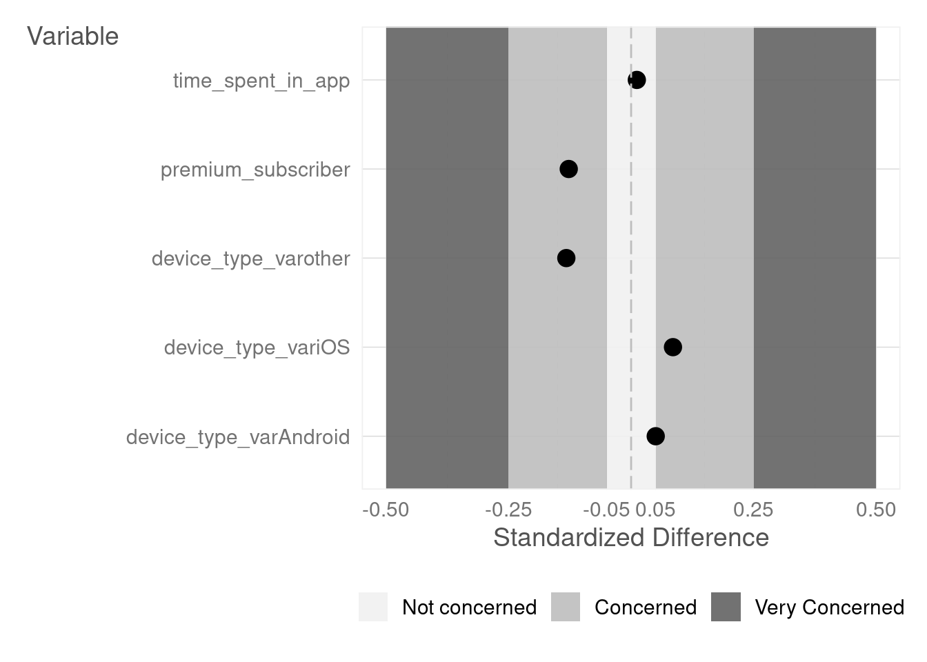
The general rule of thumb is that an absolute effect size greater than 0.25 signals a lack of baseline equivalence, and statistical adjustments are unlikely to fully remedy the situation. If the absolute effect size lies between 0.05 and 0.25, statistical adjustments become necessary. An absolute effect size below 0.05 indicates strong evidence of baseline equivalence.

3.2 Linking Baseline Equivalence to Potential Outcomes

The concept of baseline equivalence is intimately connected to the potential outcomes framework we discussed in Section 2.1. Baseline equivalence supports the crucial ignorability assumption in the potential outcomes framework, which states that treatment assignment is independent of the potential outcomes given observed covariates. When groups are equivalent at baseline, it’s more plausible that any differences in outcomes are due to the treatment rather than unobserved confounders.

By striving for baseline equivalence, we’re essentially attempting to create conditions that allow us to more accurately estimate the causal effects defined in the potential outcomes framework. This connection underscores the importance of assessing and establishing baseline equivalence in any causal inference study, whether experimental or observational.

3.3 The {im} Package in R

The R package {im} package provides a convenient way to check baseline equivalence using the im::checkBaseline function and visualize the results with im::balancePlot.

set.seed(123)
data <- data.frame(
  time_spent_in_app = rnorm(1000, mean = 60, sd = 15),
  # Continuous
  premium_subscriber = rbinom(1000, 1, 0.2),
  # Binary
  device_type = factor(sample(
    c("iOS", "Android", "other"), 1000, replace = TRUE
  )),
  # Factor
  treatment = factor(sample(c(
    "control", "treatment"
  ), 1000, replace = TRUE))
)

# Check baseline equivalence
baseline_results <- im::checkBaseline(
  data,
  variables = c("time_spent_in_app", "premium_subscriber", "device_type"),
  treatment = "treatment"
)

im::balancePlot(data = baseline_results)

3.4 The Importance of Baseline Equivalence

Whether your study design is experimental or observational, the principle of baseline equivalence should always be top of mind. It’s a fundamental building block for drawing valid causal inferences.

Remember, we can only assess baseline equivalence for the characteristics we can measure. It’s crucial to consider the possibility of unobservable factors that might differ between groups at baseline and potentially bias our findings. By acknowledging and addressing these potential confounders, we strengthen the rigor and reliability of our causal analyses.

Learn more

WWC (2020) What Works Clearinghouse Baseline Equivalence Standard.
Anderson and Maxwell (2018) Baseline Equivalence: What it is and Why it is Needed.

--- title: "Baseline Equivalence" share: permalink: "https://book.martinez.fyi/baseline.html" description: "Business Data Science: What Does it Mean to Be Data-Driven?" linkedin: true email: true mastodon: true --- ![Baseline Equivalence](img/baseline.jpg){.lightbox} In the quest to discern the true impact of an intervention, we must first establish a level playing field. The concept of **baseline equivalence** serves this purpose, ensuring that the groups under comparison are similar enough in key observed characteristics before the intervention takes place. Any discrepancies at baseline could muddy the waters, making it difficult to isolate the intervention's effect from pre-existing differences. Baseline equivalence is particularly crucial in scenarios where sample sizes are small or when we're dealing with observational studies. Let's say a company wants to evaluate a new algorithm designed to boost user engagement. If the group exposed to this new algorithm (the treatment group) already exhibited higher engagement levels than the control group prior to the experiment, any observed increase could simply be a continuation of their existing behavior, not necessarily a testament to the algorithm's effectiveness. ## Gauging Baseline Equivalence {#sec-baseline} To ascertain baseline equivalence, we turn to pre-intervention outcomes and other relevant observables. A common approach is to calculate the **effect size**, a standardized measure of the magnitude of an effect. For **continuous variables**, Hedges' g statistic is a popular choice (@hedges1981distribution): $$ g = \frac{\omega(y_t-y_c)}{\sqrt{\frac{(n_t - 1) s_t^2 + (n_c - 1) s_c^2}{n_t+n_c - 2}}} $$ where - $y_t$ is the mean for the treatment group - $y_c$ is the mean for the comparison group - $n_t$ is the sample size for the treatment group - $n_c$ is the sample size for the comparison group - $s_t$ is the standard deviation for the treatment group - $s_c$ is the standard deviation for the comparison group - $\omega := 1 - \frac{3}{4(n_t+n_c)-9}$ is the small sample size correction. For **binary outcomes**, Cox's index comes into play (see @cox1972regression): $$ d = \omega \left[ \ln\left(\frac{p_t}{1-p_t}\right) - \ln\left(\frac{p_c}{1-p_c}\right) \right] $$ where: - $p_t$ is the the mean of the outcome in the intervention group - $p_c$ is the mean of the outcome in the comparison group - $\omega := 1 - \frac{3}{4(n_t+n_c)-9}$ is the small sample size correction. The general rule of thumb is that an absolute effect size greater than 0.25 signals a lack of baseline equivalence, and statistical adjustments are unlikely to fully remedy the situation. If the absolute effect size lies between 0.05 and 0.25, statistical adjustments become necessary. An absolute effect size below 0.05 indicates strong evidence of baseline equivalence. ## Linking Baseline Equivalence to Potential Outcomes The concept of baseline equivalence is intimately connected to the potential outcomes framework we discussed in @sec-potential. Baseline equivalence supports the crucial ignorability assumption in the potential outcomes framework, which states that treatment assignment is independent of the potential outcomes given observed covariates. When groups are equivalent at baseline, it's more plausible that any differences in outcomes are due to the treatment rather than unobserved confounders. By striving for baseline equivalence, we're essentially attempting to create conditions that allow us to more accurately estimate the causal effects defined in the potential outcomes framework. This connection underscores the importance of assessing and establishing baseline equivalence in any causal inference study, whether experimental or observational. ## The {im} Package in R The R package {im} package provides a convenient way to check baseline equivalence using the `im::checkBaseline` function and visualize the results with `im::balancePlot`. ```{r baseline} set.seed(123) data <- data.frame( time_spent_in_app = rnorm(1000, mean = 60, sd = 15), # Continuous premium_subscriber = rbinom(1000, 1, 0.2), # Binary device_type = factor(sample( c("iOS", "Android", "other"), 1000, replace = TRUE )), # Factor treatment = factor(sample(c( "control", "treatment" ), 1000, replace = TRUE)) ) # Check baseline equivalence baseline_results <- im::checkBaseline( data, variables = c("time_spent_in_app", "premium_subscriber", "device_type"), treatment = "treatment" ) im::balancePlot(data = baseline_results) ``` ## The Importance of Baseline Equivalence Whether your study design is experimental or observational, the principle of baseline equivalence should always be top of mind. It's a fundamental building block for drawing valid causal inferences. Remember, we can only assess baseline equivalence for the characteristics we can measure. It's crucial to consider the possibility of unobservable factors that might differ between groups at baseline and potentially bias our findings. By acknowledging and addressing these potential confounders, we strengthen the rigor and reliability of our causal analyses. ::: {.callout-tip} ## Learn more - @wwc_baseline What Works Clearinghouse Baseline Equivalence Standard. - @anderson2018baseline Baseline Equivalence: What it is and Why it is Needed. :::