---
title: "Bayes 101"
filters:
- shinylive
---
<img src="img/bayes.webp" align="right" height="280" alt="Bayes 101" />
In the bustling marketplace of ideas that is modern data science, Bayesian
statistics stands out as a powerful and intuitive approach to understanding
uncertainty and making decisions. For business data scientists, it offers a
flexible framework that naturally incorporates prior knowledge, updates beliefs
based on new evidence, and quantifies uncertainty in a way that's both
mathematically rigorous and intuitively appealing.
Now, let's set some expectations. To truly thrive as a business data scientist,
you'll need more than a passing familiarity with statistics. Think of it this
way: an analyst knows how to use a calculator, while a data scientist knows how
that calculator works—and can even build one from scratch to tackle the specific
problem at hand. Let me be clear: this chapter isn't a course in calculator
construction. We won't delve into the nuts and bolts of how it's built, or even
all the inner workings. Instead, our aim is to convince you that this particular
calculator is worth learning more about. We want to spark your curiosity, to
show you why this tool deserves a prime spot in your data science toolbox.
In this chapter, we'll explore the basics of Bayesian statistics, delve into
Bayes' rule, and examine why this paradigm is particularly well-suited for
business applications.
## The Essence of Bayesian Thinking
At its core, Bayesian statistics is about updating our beliefs in light of new
evidence. This process mirrors how we often think about problems in business: we
start with some prior knowledge or assumptions, gather data, and then update our
understanding based on what we've learned.
As @kruschke2018bayesian eloquently put it, "The main idea of Bayesian analysis
is simple and intuitive. There are some data to be explained, and we have a set
of candidate explanations. Before knowing the new data, the candidate
explanations have some prior credibilities of being the best explanation. Then,
when given the new data, we shift credibility toward the candidate explanations
that better account for the data, and we shift credibility away from the
candidate explanations that do not account well for the data."
This perspective highlights a fundamental principle of Bayesian analysis: it's a
process of reallocating credibility across possibilities. In a business context,
these "possibilities" might be different strategies, market scenarios, or
parameter values in a model. As we gather more data, we adjust our beliefs about
which possibilities are more or less likely to be true.
The Bayesian approach contrasts with the more traditional frequentist statistics
in a fundamental way. While frequentists treat parameters as fixed (but unknown)
quantities and data as random, Bayesians view parameters as random variables and
data as fixed once observed. This shift in perspective leads to more intuitive
interpretations of statistical results and allows for the incorporation of prior
knowledge into our analyses.
## Bayes' Rule: The Heart of Bayesian Statistics
The cornerstone of Bayesian statistics is Bayes' rule, named after the Reverend
Thomas Bayes. This elegant formula shows us how to update probabilities when we
receive new information. In its simplest form, Bayes' rule is expressed as:
$$
P(A|B) = \frac{P(B|A)P(A)}{P(B)}
$$
Where:
- $P(A|B)$ is the posterior probability of A given B
- $P(B|A)$ is the likelihood of B given A
- $P(A)$ is the prior probability of A
- $P(B)$ is the marginal likelihood of B
In the context of parameter estimation, which is often our goal in business data
science, we can rewrite Bayes' rule as:
$$
P(\theta|D) = \frac{P(D|\theta)P(\theta)}{P(D)}
$$
Where:
- $\theta$ represents our parameter(s) of interest
- $D$ represents our observed data
- $P(\theta|D)$ is the posterior distribution of our parameter given the data
- $P(D|\theta)$ is the likelihood of the data given the parameter
- $P(\theta)$ is our prior distribution for the parameter
- $P(D)$ is the marginal likelihood of the data
This formulation clearly illustrates the process of reallocating credibility. We
start with our prior beliefs about the parameters $P(\theta)$, consider how
likely the data are given those parameters $P(D|\theta)$, and end up with an
updated (posterior) belief about the parameters $P(\theta|D)$.
## The Case of the Declining User Engagement
Even if you haven't formally studied Bayesian statistics, your brain is already
wired to think like a Bayesian. To illustrate how this intuitive approach can be
applied to real-world business problems, let's consider a scenario that data
scientists in the tech sector frequently encounter: investigating a sudden
decline in user engagement and its potential impact on revenue.
Imagine you're a business data scientist at a high-growth tech company that
offers a subscription-based productivity app. You've noticed a concerning trend:
daily active users (DAU) have dropped by 15% over the past month, and this is
starting to affect revenue. Your task is to identify the most likely cause of
this engagement drop and recommend actions to reverse the trend.
Let's say we have four main hypotheses for the cause of the declining
engagement:
1. A recent feature update (Feature)
2. Increased competition in the market (Competition)
3. Seasonal variation (Seasonality)
4. Changes in marketing spend (Marketing)
Before diving into the data, you have some prior beliefs about the likelihood of
each cause, based on your experience and industry knowledge:
- Feature: 35% (feature updates can sometimes negatively impact user
experience)
- Competition: 25% (the market is becoming more saturated)
- Seasonality: 20% (there's often a summer slowdown in productivity app usage)
- Marketing: 20% (marketing budgets have been fluctuating)
This is your prior distribution. Now, as you investigate, you gather evidence:
1. User feedback shows mixed reactions to the recent feature update, with some
users reporting confusion about the new interface.
2. Market research indicates that while a major competitor launched a new
product, it hasn't gained significant market share yet.
3. Historical data shows a similar dip in engagement during the same period
last year, though not as pronounced.
4. Marketing spend has remained consistent over the past quarter.
As you collect this evidence, you update your beliefs about the likelihood of
each cause. This is where Bayesian reasoning comes into play, allowing you to
reallocate credibility based on the new information.
After considering the evidence, you might update your beliefs as follows:
- Feature: 60% (user feedback suggests this is a significant factor)
- Competition: 8% (less likely given the market research)
- Seasonality: 30% (historical data supports this as a contributing factor)
- Marketing: 2% (unlikely given consistent spend)
This is your posterior distribution. You've reallocated credibility based on the
evidence, increasing your belief that the feature update and seasonality are the
primary causes of the engagement drop.
## Communicating Uncertainty: Credible Intervals vs. Confidence Intervals
In Bayesian statistics, we often express our uncertainty about an estimated
parameter using **credible intervals.** A 95% credible interval, for example, is
a range of values that we believe, with 95% probability, contains the true value
of the parameter. This interpretation is quite intuitive and aligns well with
how we naturally think about uncertainty.
It's important to contrast credible intervals with confidence intervals, which
are frequently misinterpreted [@hoekstra2014robust]. While both express
uncertainty, their interpretations differ:
- A 95% confidence interval is constructed such that, if we were to repeat the
experiment many times, 95% of the intervals we calculate would contain the
true parameter value. This interpretation is somewhat less intuitive and
focuses on the long-run behavior of the procedure rather than the specific
interval at hand.
- A 95% credible interval, on the other hand, directly states that there's
a 95% probability that the true parameter value lies within this particular
interval, given the observed data and our prior beliefs.
In summary:
| **Feature** | **Confidence Interval** | **Credible Interval** |
|:---------------:|:-----------------------:|:----------------------------:|
| Philosophy | Frequentist | Bayesian |
| Interpretation | Repeated sampling | Probability of the parameter |
| Prior knowledge | Not used | Can be incorporated |
| Statement about | The interval itself | The parameter |
### Analogy
Imagine you're trying to estimate the height of a tree.
- **Confidence interval:** You take multiple measurements from different
angles and use them to construct an interval. You say, "If I repeated this
process many times, 95% of the intervals I create would contain the tree's
true height."
- **Credible interval:** You consider your previous knowledge about trees in
the area, combine it with your measurements, and say, "Based on my
measurements and what I already know, there's a 95% probability that the
tree's height is between X and Y meters." Credible intervals provide a more
intuitive and direct interpretation of uncertainty about a parameter.
However, they require specifying prior distributions, which can be
subjective. Confidence intervals, while less intuitive, are widely used and
don't require prior information.
### Beyond Intervals: Posterior Probabilities for Tailored Insight
Though credible intervals offer a convenient snapshot of uncertainty, they might
not always be the optimal tool to inform decisions. Let's consider a scenario
where we're assessing whether an intervention's impact surpasses a specific
threshold. This threshold could be zero – indicating whether the intervention
has any effect at all – or it could be any other relevant value, depending on
the decision at hand.
In the Bayesian framework, we can bypass the limitations of intervals and
compute the probability of the impact exceeding our threshold directly from the
posterior distribution. We simply determine the proportion of the distribution
that lies beyond the threshold. This gives us the posterior probability that the
parameter of interest is greater than our chosen value, providing a clear and
actionable insight.
It's worth noting that we might have multiple thresholds relevant to different
decisions. For example, we might be interested in the probability that the
impact is at least 'moderately' large, or the probability that it is
'substantially' large. The Bayesian approach allows us to calculate these
probabilities directly from the posterior, tailoring our uncertainty
quantification to the specific decision context.
## The Case of Karl Broman's Socks: A Bayesian Adventure in Tiny Data
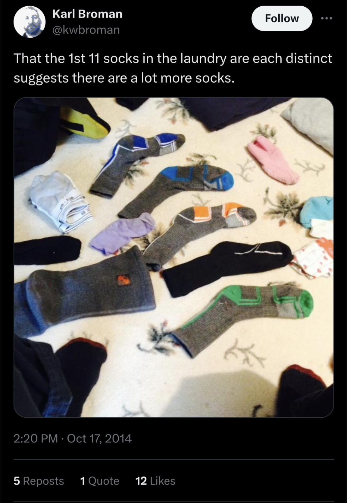{fig-alt="[Karl Broman's Socks](https://x.com/kwbroman/status/523221976001679360)" fig-align="center" width=50%}
To illustrate the power of Bayesian thinking, even with limited data, let's
consider an intriguing example from Rasmus Bååth's Blog, which he calls "Tiny
Data, Approximate Bayesian Computation and the Socks of Karl Broman" (see
[original blog
post](https://www.sumsar.net/blog/2014/10/tiny-data-and-the-socks-of-karl-broman/)).
The problem is deceptively simple: Given that [Karl Broman has 11 unique socks
in his laundry](https://x.com/kwbroman/status/523221976001679360), how many
socks does he have in total? This is a perfect example of what Bååth calls "Tiny
Data" - a situation where we have very limited information but still need to
make an inference. It's a scenario that business data scientists often face,
where decisions need to be made with incomplete information.
### The Bayesian Approach to the Sock Problem
Bååth tackles this problem using Approximate Bayesian Computation (ABC), an
intuitive albeit computationally intensive method (see @rubin1984bayesianly).
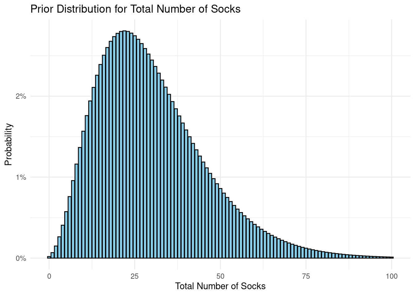
In this Bayesian adventure, we begin with two crucial pieces of information,
encoded as prior probability distributions. The number of socks is a count
variable, so we'll employ a negative binomial data generating process. (We delve
into this topic in more detail in @sec-negative-binomial.) For now, let's follow
Bååth's lead and set ($\mu = 30$) and (size = 4).
```{r prior_socks}
library(ggplot2)
# Dataframe of possible sock counts
sock_counts <- data.frame(n_socks = 0:100)

# Calculate probabilities from the negative binomial distribution
sock_counts$probability <- dnbinom(sock_counts$n_socks, mu = 30, size = 4)

# Create the histogram
ggplot(sock_counts, aes(x = n_socks, y = probability)) +
  geom_col(fill = "skyblue", color = "black") +
  scale_y_continuous(labels = scales::percent) +
  theme_minimal() +
  labs(x = "Total Number of Socks", y = "Probability") +
  ggtitle("Prior Distribution for Total Number of Socks")
```
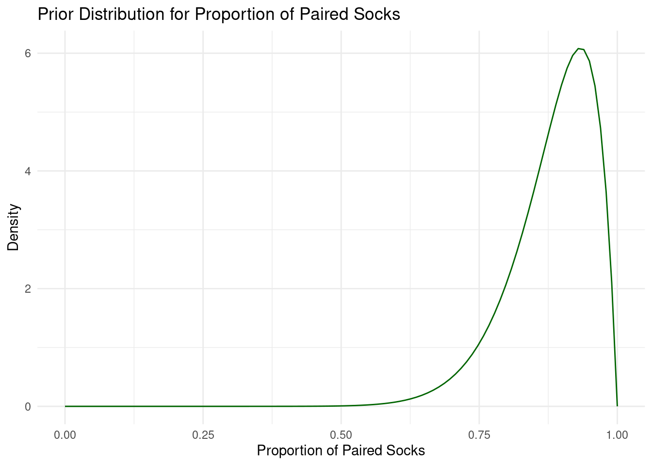
Next, we need to specify our beliefs about the proportion of socks that have a
pair. For this, we can use a beta data generating process. To remain consistent
with the blog post, we'll set shape1 = 15 and shape2 = 2. This distribution is
skewed towards higher values, suggesting a belief that most socks in a laundry
pile are likely to be paired. The parameters indicate an expectation
around 0.88, reflecting the common experience that unmatched socks are less
frequent.
```{r prior_prop}
# Create a sequence of proportions from 0 to 1
proportions <- seq(0, 1, length.out = 100)

# Calculate density values from the beta distribution
density_values <- dbeta(proportions, shape1 = 15, shape2 = 2)

# Create the density plot
ggplot(data.frame(proportion = proportions, density = density_values),
       aes(x = proportion, y = density)) +
  geom_line(color = "darkgreen") +
  theme_minimal() +
  labs(x = "Proportion of Paired Socks", y = "Density") +
  ggtitle("Prior Distribution for Proportion of Paired Socks")
```
These prior distributions encapsulate our initial beliefs before we observe any
data. The Bayesian approach elegantly allows us to update these beliefs based on
the evidence, leading to more informed posterior distributions.
Now, let's craft the R code for simulating draws from this data generating
process.
```{r simulation, message=FALSE, warning=FALSE}
library(dplyr)
library(furrr)
library(patchwork)

set.seed(123)

# Enable parallel processing with the number of cores available
plan(multisession, workers = availableCores())

# Define the number of socks picked
n_picked <- 11

# Improved simulation function
simulate_socks <- function(n_picked) {
  # Generate total number of socks from prior
  n_socks <- rnbinom(1, mu = 30, size = 4)

  # Generate proportion of paired socks from prior
  prop_pairs <- rbeta(1, shape1 = 15, shape2 = 2)

  # Calculate number of pairs and odd socks
  n_pairs <- round(floor(n_socks / 2) * prop_pairs)
  n_odd <- n_socks - n_pairs * 2

  # Simulate picking socks
  socks <- rep(seq_len(n_pairs + n_odd), rep(c(2, 1), c(n_pairs, n_odd)))
  picked_socks <- sample(socks, size = min(n_picked, n_socks))
  sock_counts <- table(picked_socks)

  # Return results
  tibble(
    unique = sum(sock_counts == 1),
    pairs = sum(sock_counts == 2),
    n_socks = n_socks,
    n_pairs = n_pairs,
    n_odd = n_odd,
    prop_pairs = prop_pairs
  )
}

# Run simulations
n_sims <- 100000
sock_sim <- future_map_dfr(1:n_sims, ~simulate_socks(n_picked),
                           .options = furrr_options(seed = 123))

# Filter for matching simulations (11 unique socks, 0 pairs)
post_samples <- sock_sim %>%
  filter(unique == 11, pairs == 0)
```
This code implements the ABC method, which is a perfect illustration of the
"reallocation of credibility across possibilities" that Kruschke and Liddell
describe:
1. We define prior distributions for the total number of socks (negative
binomial) and the proportion of paired socks (beta). These represent our
initial beliefs about the possibilities.
2. We create a generative model that simulates picking socks from a laundry
pile.
3. We run this simulation many times (100,000 in this case), each time
generating a possible scenario.
4. We keep only those simulations that match our observed data (11 unique
socks, 0 pairs). This step is where we reallocate credibility, focusing on
the possibilities that are consistent with our observation.
5. We analyze the results by calculating median values from the retained
samples, which represent our updated beliefs.
### Visualizing the Results
```{r viz}
# Prepare data for plotting
prior_data <- sock_sim %>%
  count(n_socks) %>%
  mutate(prop = n / sum(n),
         type = "Prior")

posterior_data <- post_samples %>%
  count(n_socks) %>%
  mutate(prop = n / sum(n),
         type = "Posterior")

plot_data <- bind_rows(prior_data, posterior_data)

# Plot prior and posterior distributions
p1 <- ggplot(plot_data, aes(x = n_socks, y = prop, fill = type)) +
  geom_col(position = "dodge", alpha = 0.7) +
  scale_fill_manual(values = c("Prior" = "lightgreen", "Posterior" = "skyblue")) +
  labs(title = "Prior and Posterior Distributions of Total Socks",
       x = "Number of Socks", y = "", fill = "Distribution") +
  theme_minimal() +
  theme(legend.position = "top")

# Plot the posterior distribution of pairs and odd socks
p2 <- ggplot(post_samples, aes(x = n_pairs, y = n_odd)) +
  geom_hex(bins = 30) +
  scale_fill_viridis_c() +
  labs(title = "Joint Posterior Distribution of Pairs and Odd Socks",
       x = "Number of Pairs", y = "Number of Odd Socks") +
  theme_minimal()

# Combine plots
p1 / p2
```
### Results and Interpretation
After running this model, our best guess (median of the posterior) is that Karl
Broman has approximately:
```{r summary}
# Calculate summary statistics
summary_stats <- post_samples %>%
  summarize(
    median_socks = median(n_socks),
    median_pairs = median(n_pairs),
    median_odd = median(n_odd),
    ci_lower_socks = quantile(n_socks, 0.025),
    ci_upper_socks = quantile(n_socks, 0.975)
  )
```
- Total socks: `r summary_stats$median_socks`
(95% CI: `r summary_stats$ci_lower_socks` - `r summary_stats$ci_upper_socks`)
- Pairs of socks: `r summary_stats$median_pairs`
- Odd socks: `r summary_stats$median_odd`
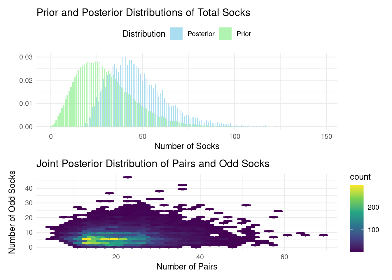
Remarkably, when Karl later revealed the actual numbers, it turned out there
were 21 pairs and 3 odd socks, totaling 45 socks. The estimate is surprisingly
close, considering we only had one piece of information to work with! The
visualizations provide additional insights:
The first plot shows how our beliefs about the total number of socks changed
from the prior (green) to the posterior (blue) distribution after incorporating
the data. This is a clear visualization of the reallocation of credibility
across possibilities. The second plot illustrates the joint posterior
distribution of pairs and odd socks, showing the range of plausible combinations
given our model and data.
This example beautifully illustrates several key aspects of Bayesian thinking:
1. Incorporation of prior knowledge: The model uses reasonable priors based on
general knowledge about sock ownership.
2. Handling uncertainty: The posterior distribution provides a range of
plausible values, not just a point estimate.
3. Learning from limited data: Even with just one piece of information (11
unique socks), we can make a surprisingly accurate inference.
4. Flexibility: The ABC approach allows us to work with a complex model that
would be difficult to handle with traditional methods.
5. Reallocation of credibility: We start with a wide range of possibilities and
narrow down to those most consistent with our observation.
In business contexts, we often face similar situations - limited data combined
with domain expertise or prior experience. The sock example, while whimsical,
demonstrates how Bayesian methods can be powerful in such real-world scenarios.
As we progress through this book, we'll explore how these principles can be
applied to more complex business problems.
As Kruschke and Liddell (2018) point out, one of the key advantages of Bayesian
analysis is that "the posterior distribution can be directly examined to see
which parameter values are most credible, and what range of parameter values
covers the most credible values." This direct interpretation is particularly
valuable in business settings, where we often need to communicate results to
non-technical stakeholders.
For instance, in our sock example, we can straightforwardly say that
"there's a 95% probability that the total number of socks is between
`r summary_stats$ci_lower_socks` and `r summary_stats$ci_upper_socks`."
This statement is intuitive and directly addresses the uncertainty in our
estimate, which is crucial for informed decision-making.
Additionally, we can quantify probabilities for specific scenarios, such as:
"The probability that there are at least 15 pairs
is `r scales::percent(mean(post_samples$n_pairs > 14))`."
Moreover, Bayesian methods naturally handle the "small data" scenarios that are
common in business. While big data gets a lot of attention, many important
business decisions are made with limited information. The Bayesian framework
allows us to start with prior knowledge (perhaps based on industry benchmarks or
previous experience), update this with whatever data is available, and still
produce meaningful results.
### A Note on Priors
It's important to remember that the less data you have, the more influential
your priors become. Transparency about your priors is essential, as is
investigating the sensitivity of your findings to different prior choices.
However, don't shy away from using informative priors when justified by data.
The interactive dashboard below utilizes {shinylive} (see @shinylive) to run
these simulations directly in your browser, allowing you to experiment with
various priors and observe their impact.
```{shinylive-r}
#| standalone: true
#| viewerHeight: 800
library(shiny)
library(ggplot2)
library(dplyr)
library(furrr)
library(shinybusy)
library(shinydashboard)

# Enable parallel processing with the number of cores available
plan(multisession, workers = availableCores())

# Define the number of socks picked
n_picked <- 11

simulate_socks <- function(n_picked, mu, size, shape1, shape2) {
  # Generate total number of socks from prior
  n_socks <- rnbinom(1, mu = mu, size = size)

  # Generate proportion of paired socks from prior
  prop_pairs <- rbeta(1, shape1 = shape1, shape2 = shape2)

  # Calculate number of pairs and odd socks
  n_pairs <- round(floor(n_socks / 2) * prop_pairs)
  n_odd <- n_socks - n_pairs * 2

  # Simulate picking socks
  socks <- rep(seq_len(n_pairs + n_odd), rep(c(2, 1), c(n_pairs, n_odd)))
  picked_socks <- sample(socks, size = min(n_picked, n_socks))
  sock_counts <- table(picked_socks)

  # Return results
  tibble(
    unique = sum(sock_counts == 1),
    pairs = sum(sock_counts == 2),
    n_socks = n_socks,
    n_pairs = n_pairs,
    n_odd = n_odd,
    prop_pairs = prop_pairs
  )
}

ui <- dashboardPage(
  skin = "black",
  dashboardHeader(title = "Karl's Socks"),
  dashboardSidebar(
    numericInput(
      inputId = "seed",
      label = "Random Seed",
      value = 123,
      min = 1,
      step = 1
    ),
    numericInput(
      inputId = "n_sims",
      label = "Number of Simulations",
      value = 10000,
      min = 100,
      step = 100
    ),
    sliderInput(
      inputId = "mu",
      label = "mu",
      min = 15,
      max = 60,
      value = 40,
      step = 1
    ),
    sliderInput(
      inputId = "size",
      label = "Size",
      min = 3,
      max = 10,
      value = 4,
      step = 1
    ),
    sliderInput(
      inputId = "shape1",
      label = "Shape 1",
      min = 2,
      max = 20,
      value = 15,
      step = 1
    ),
    sliderInput(
      inputId = "shape2",
      label = "Shape 2",
      min = 2,
      max = 8,
      value = 2,
      step = 1
    ),
    actionButton("run_sim", "Run Simulation")
  ),
  dashboardBody(
    use_busy_spinner(spin = "fading-circle"),
    fluidRow(
      box(
        title = "Prior Distribution for Total Number of Socks",
        status = "danger", solidHeader = TRUE,
        collapsible = TRUE,
        plotOutput("prior_socks")
      ),

      box(
        title = "Prior Distribution for Proportion of Paired Socks",
        status = "danger", solidHeader = TRUE,
        collapsible = TRUE,
        plotOutput("prior_prop")
      )
    ),

    fluidRow(
      box(
        title = "Prior and Posterior Distributions of Total Socks",
        status = "danger", solidHeader = TRUE,
        collapsible = TRUE,
        plotOutput("distribution_plot")
      ),

      box(
        title = "Joint Posterior Distribution of Pairs and Odd Socks",
        status = "danger", solidHeader = TRUE,
        collapsible = TRUE,
        plotOutput("joint_plot")
      )
    ),

    fluidRow(
      valueBoxOutput("pr_pairs")
    )
  )
)

server <- function(input, output) {

  sock_sim <- eventReactive(input$run_sim, {
    show_modal_spinner()
    on.exit(remove_modal_spinner())
    set.seed(input$seed)
    local_mu <- input$mu
    local_size <- input$size
    local_shape1 <- input$shape1
    local_shape2 <- input$shape2
    future_map_dfr(1:input$n_sims,
                   ~simulate_socks(n_picked = 11,
                                   mu = local_mu,
                                   size = local_size,
                                   shape1 = local_shape1,
                                   shape2 = local_shape2),
                   .options = furrr_options(seed = 123))
  })

  # Filter for matching simulations (11 unique socks, 0 pairs)
  post_samples <- reactive({
    sock_sim() %>%
      filter(unique == 11, pairs == 0)
  })

  output$pr_pairs <- renderValueBox({
    req(post_samples())
    valueBox(
      scales::percent(mean(post_samples()$n_pairs > 14)),
      "Pr[# Pairs > 14]", icon = icon("socks"),
      color = "red"
    )
  })

  # Prepare data for plotting
  prior_data <- reactive({
    sock_sim() %>%
      count(n_socks) %>%
      mutate(prop = n / sum(n),
             type = "Prior")
  })

  posterior_data <- reactive({
    if(nrow(post_samples()) == 0) {
      return(tibble(n_socks = numeric(), prop = numeric(), type = character()))
    }
    post_samples() %>%
      count(n_socks) %>%
      mutate(prop = n / sum(n),
             type = "Posterior")
  })

  output$prior_socks <- renderPlot({
    # Dataframe of possible sock counts
    sock_counts <- data.frame(n_socks = 0:100)

    # Calculate probabilities from the negative binomial distribution
    sock_counts$probability <- dnbinom(sock_counts$n_socks,
                                       mu = input$mu,
                                       size = input$size)

    # Create the histogram
    ggplot(sock_counts, aes(x = n_socks, y = probability)) +
      geom_col(fill = "skyblue", color = "black")+
      scale_y_continuous(labels = scales::percent) +
      theme_minimal() +
      labs(x = "Total Number of Socks", y = "Probability")
  })

  output$prior_prop <- renderPlot({
    # Create a sequence of proportions from 0 to 1
    proportions <- seq(0, 1, length.out = 100)

    # Calculate density values from the beta distribution
    density_values <- dbeta(proportions, shape1 = input$shape1,
                            shape2 = input$shape2)

    # Create the density plot
    ggplot(data.frame(proportion = proportions, density = density_values),
           aes(x = proportion, y = density)) +
      geom_line(color = "darkgreen") +
      theme_minimal() +
      labs(x = "Proportion of Paired Socks", y = "Density")
  })

  output$distribution_plot <- renderPlot({
    req(prior_data(), posterior_data())
    plot_data <- bind_rows(prior_data(), posterior_data())

    ggplot(plot_data, aes(x = n_socks, y = prop, fill = type)) +
      geom_col(position = "dodge", alpha = 0.7) +
      scale_fill_manual(values = c("Prior" = "lightgreen", "Posterior" = "skyblue")) +
      scale_y_continuous(labels = scales::percent) +
      labs(x = "Number of Socks", y = "Probability", fill = "Distribution") +
      theme_minimal() +
      theme(legend.position = "top")
  })

  output$joint_plot <- renderPlot({
    req(post_samples())
    if(nrow(post_samples()) > 0) {
      ggplot(post_samples(), aes(x = n_pairs, y = n_odd)) +
        geom_hex(bins = 30) +
        scale_fill_viridis_c() +
        labs(x = "Number of Pairs", y = "Number of Odd Socks") +
        theme_minimal()
    } else {
      ggplot() +
        annotate("text", x = 0.5, y = 0.5, label = "No matching simulations found") +
        theme_void()
    }
  })
}

shinyApp(ui, server)
```
## Conclusion
Bayesian statistics offers a powerful and intuitive framework for business data
science, aligning closely with how businesses make decisions. By incorporating
prior knowledge, we can update our beliefs based on evidence and quantify
uncertainty in a natural way. The concept of reallocating credibility across
possibilities provides an intuitive way to think about learning from data.
Furthermore, Bayesian methods are particularly well-suited to the "small data"
scenarios often encountered in business. While "big data" garners much
attention, many crucial business decisions hinge on limited information. The
Bayesian framework allows us to begin with prior knowledge, update it with
available data, and then communicate our findings in plain language.
In essence, Bayesian statistics provides a flexible and powerful approach for
tackling the complex and often uncertain world of business decision-making.
::: {.callout-tip}
## Learn more
- @kruschke2018bayesian Bayesian data analysis for newcomers.
- @mcelreath2018statistical Statistical Rethinking: A Bayesian Course with
Examples in R and Stan
- @gelman2013bayesian Bayesian Data Analysis.
:::

](img/socks.png)