11  Randomized Encouragement Design

Nudge

In the dynamic world of business, a recurring question is, “What if our users took a particular action? What would be the impact?” Yet, randomly assigning users to specific behaviors—forcing their hand, so to speak—isn’t feasible. The most effective approach in such situations is a Randomized Encouragement Design (RED), a clever method rooted in the econometric concept of instrumental variables. In a RED, a subset of users is randomly nudged towards the action in question.

The history of instrumental variables is itself a fascinating tale, originating in the 1920s with economist Philip Wright. Surprisingly, it first appeared in an appendix to his book on tariffs for animal and vegetable oils. While the book itself didn’t make a big splash, the appendix held a groundbreaking solution to the identification problem in economics. Interestingly, there’s some debate among historians about whether it was Philip Wright himself or his son, the renowned geneticist Sewall Wright, who actually developed the concept. Regardless of its exact origin, this approach, instrumental variables, even played a pivotal role in the research that earned Joshua Angrist and Guido Imbens the 2021 Nobel Prize in Economics.

11.1 Understanding REDs: Compliance and Potential Outcomes

REDs hinge on understanding how users respond to encouragement, categorizing them into four groups:

• Compliers: Those who change their behavior based on encouragement.
• Always-takers: Those who would take the action regardless of encouragement.
• Never-takers: Those who wouldn’t take the action regardless of encouragement.
• Defiers: (Rarely assumed to exist) Do the opposite of what’s encouraged. While theoretically possible, this group is often assumed away in most analyses for simplicity.

The potential outcomes framework is crucial for understanding these designs. For each participant, we consider:

• \(Y(1)\): The outcome if encouraged
• \(Y(0)\): The outcome if not encouraged
• \(D(1)\): The treatment status if encouraged
• \(D(0)\): The treatment status if not encouraged

11.2 What We Want to Know: ITT and CACE

In the world of REDs, our curiosity often leads us down two paths:

1. Intent-to-Treat (ITT) Effect: Sometimes, we’re primarily interested in the value of the encouragement itself—the gentle push, the subtle prompt, the enticing incentive. In this case, we estimate the Intent-to-Treat (ITT) effect: the average change in the outcome simply due to being encouraged, regardless of whether individuals actually comply and take the action. Mathematically, this is represented as: \[ITT = E[Y(1) - Y(0)]\] For example, a marketing team might want to know the overall impact of sending a promotional email, regardless of whether recipients actually click through and make a purchase.

2. Complier Average Causal Effect (CACE): In other scenarios, our focus shifts to the true causal impact of the action itself. We want to know what happens when people actually take that step, change that behavior, or adopt that product. This is where the Complier Average Causal Effect (CACE), also known as the Local Average Treatment Effect (LATE), comes in. It isolates the average effect of the treatment specifically for those who are swayed by the encouragement—the compliers. The CACE is defined as: \[CACE = E[Y(1) - Y(0)|D(1) = 1, D(0) = 0]\] where \(Z\) is the encouragement assignment and \(D\) is the actual treatment received. For instance, a product team might be interested in the impact of actually using a new feature on user engagement, rather than just being encouraged to use it.

11.3 Making it Work: Key Assumptions

For REDs to yield valid causal conclusions, a few key assumptions need to hold true:

1. Ignorability of the instrument: The encouragement assignment is random and independent of potential outcomes. This ensures that any differences we observe are due to the encouragement, not pre-existing differences between groups.
2. Exclusion restriction: Encouragement affects the outcome only through its effect on treatment take-up. For example, receiving an email about a new feature shouldn’t directly impact user engagement; it should only impact engagement through increased feature usage.
3. Monotonicity: There are no defiers (i.e., no one does the opposite of what they’re encouraged to do). This simplifies our analysis and is usually a reasonable assumption in most business contexts.
4. Relevance: The encouragement actually affects treatment take-up (i.e., there are compliers). If our encouragement doesn’t change anyone’s behavior, we can’t learn anything about the treatment effect

Violations of these assumptions can lead to biased estimates. For example, if the exclusion restriction is violated (e.g., if merely receiving an email about a feature increases engagement regardless of usage), our CACE estimate will be inflated.

11.4 Practical Considerations: Designing Effective Encouragements

The success of a RED hinges on the effectiveness of the encouragement. Here are some tips for designing impactful nudges:

1. Relevance: Ensure the encouragement is relevant to the user’s context and interests.
2. Timing: Deliver the encouragement when users are most likely to be receptive.
3. Clarity: Make the encouraged action clear and easy to understand.
4. Incentives: Consider offering small incentives, but be cautious not to overly influence behavior.
5. Testing: Test different encouragement strategies to find the most effective approach.

Remember, the goal is to influence behavior enough to create a meaningful difference between encouraged and non-encouraged groups, without being coercive.

11.5 Common Pitfalls and Challenges

While REDs are powerful, they come with their own set of challenges:

1. Weak Instruments: If your encouragement isn’t very effective at changing behavior, you’ll have a “weak instrument.” This can lead to imprecise and potentially biased estimates.
2. Spillover Effects: In some cases, encouraged individuals might influence non-encouraged individuals, violating the exclusion restriction.
3. Non-Compliance: High rates of non-compliance (always-takers and never-takers) can reduce the precision of your estimates.
4. External Validity: The CACE only applies to compliers, which may not be representative of your entire user base.

11.6 Examples with synthetic data

Now, let’s dive into a practical example to illustrate how REDs work in a business context.

Imagine you work for a social media company that has just developed a new AI tool allowing creators to reach audiences regardless of their native language. This feature is computationally intensive, so you only want to maintain it if the impact of using the feature is an increase in watch time of at least 200 hours per week. How would you design an experiment to decide whether this feature should be kept available to users of your platform or discontinued?

A simple experiment in which you make the feature available to some users and not others would not answer the relevant business question because you cannot force users to use the feature, and those who choose to use it are likely fundamentally different from those who choose not to use it. Moreover, the engineering team was eager to make this available to everyone, and there’s no way you can take the feature away from people because that would be a really bad user experience.

The solution is to randomly encourage some users to use the feature. As long as the encouragement is effective, we will have a valid instrument that we can use to answer our business question. To do this, we will be using the {BIVA} R package.

Let’s start by simulating some fake data. We will borrow the code from the package vignette which generates data that works for our little story.

set.seed(1997)  # Set random seed for reproducibility
n <- 200         # Total number of individuals

# Generate Covariates:
# X: Continuous, observed covariate
X <- rnorm(n)      # Draw from standard normal distribution

# U: Binary, unobserved confounder
U <- rbinom(n, 1, 0.5)  # 1 = U = 1 with 50% probability

# Determine True Principal Strata (PS) Membership:
# 1: Complier, 2: Never-taker, 3: Always-taker
true.PS <- rep(0, n)       # Initialize PS vector
U1.ind <- (U == 1)       # Indices where U = 1
U0.ind <- (U == 0)       # Indices where U = 0
num.U1 <- sum(U1.ind)    # Number of individuals with U = 1
num.U0 <- sum(U0.ind)    # Number of individuals with U = 0

# Assign PS membership based on U:
# For U = 1: 60% compliers, 30% never-takers, 10% always-takers
# For U = 0: 40% compliers, 50% never-takers, 10% always-takers
true.PS[U1.ind] <- t(rmultinom(num.U1, 1, c(0.6, 0.3, 0.1))) %*% c(1, 2, 3)
true.PS[U0.ind] <- t(rmultinom(num.U0, 1, c(0.4, 0.5, 0.1))) %*% c(1, 2, 3)

# Assign Treatment (Z):
# Half the individuals are assigned to treatment (Z = 1), half to control (Z = 0)
Z <- c(rep(0, n / 2), rep(1, n / 2))

# Determine Treatment Received (D) Based on PS and Z:
D <- rep(0, n)            # Initialize treatment received vector

# Define indices for each group:
c.trt.ind <- (true.PS == 1) & (Z == 1)  # Compliers, treatment
c.ctrl.ind <- (true.PS == 1) & (Z == 0)  # Compliers, control
nt.ind <- (true.PS == 2)               # Never-takers
at.ind <- (true.PS == 3)               # Always-takers

# Count individuals in each group:
num.c.trt <- sum(c.trt.ind)
num.c.ctrl <- sum(c.ctrl.ind)
num.nt <- sum(nt.ind)
num.at <- sum(at.ind)

# Assign treatment received:
D[at.ind] <- rep(1, num.at)   # Always-takers receive treatment
D[c.trt.ind] <- rep(1, num.c.trt) # Compliers in treatment group receive treatment

# Generate Observed Outcome (Y):
Y <- rep(0, n) # Initialize outcome vector

# Outcome model for compliers in control group:
Y[c.ctrl.ind] <- rnorm(num.c.ctrl,
 mean = 5000 + 100 * X[c.ctrl.ind] - 300 * U[c.ctrl.ind],
 sd = 50
)

# Outcome model for compliers in treatment group:
Y[c.trt.ind] <- rnorm(num.c.trt,
 mean = 5250 + 100 * X[c.trt.ind] - 300 * U[c.trt.ind],
 sd = 50
)

# Outcome model for never-takers:
Y[nt.ind] <- rnorm(num.nt,
 mean = 6000 + 100 * X[nt.ind] - 300 * U[nt.ind],
 sd = 50
)

# Outcome model for always-takers:
Y[at.ind] <- rnorm(num.at,
 mean = 4500 + 100 * X[at.ind] - 300 * U[at.ind],
 sd = 50
)

# Create a data frame with all variables:
df <- data.frame(Y = Y, Z = Z, D = D, X = X, U = U)

The data generating process above creates a scenario with two-sided noncompliance. In other words, those encouraged to use the AI feature can choose not to do it, and those not encouraged can choose to do it. Additionally, this data generation process has no defiers, meaning the nudge works as intended but is not perfect. We have compliers, never-takers, and always-takers.

The code generates data for 200 individuals, including their compliance status and outcome. We have two baseline covariates: one observed (a continuous variable, X) and one unobserved (a binary variable, U).

The unobserved confounder U determines each individual’s membership in one of the two principal strata. An individual has a 60% probability of being a complier if U = 1, and a 30% probability if U = 0.

The outcome models vary by strata-nudge combinations. Compliers may or may not adopt the treatment depending on their assigned nudge, resulting in two distinct outcome models for the treatment groups. Never-takers, on the other hand, will never adopt the treatment, so they have a single outcome model

All three outcome models depend on both the observed \(X\) and the unobserved \(U\), with identical slopes. The difference between the intercepts of the outcome models for compliers (\(5250 - 5000 = 250\)) represents the Complier Average Causal Effect (CACE). This is the true causal effect we’re trying to estimate, but it’s hidden from us in real-world scenarios due to the presence of unobserved confounders and the inability to directly observe compliance types.

The Perils of Naive OLS Analysis

In many business settings, analysts might be tempted to use simple regression techniques to estimate causal effects. However, this approach can lead to severely biased estimates when dealing with scenarios like the one described above. Let’s explore why this is the case and how it could lead to incorrect business decisions.

Suppose we were unaware of the necessity of using instrumental variables and naively applied a linear regression to answer our question about the impact of the AI translation feature on watch time.

OLS <- lm(data = df, formula = Y ~ D + X)
broom::tidy(OLS)

# A tibble: 3 × 5
  term        estimate std.error statistic   p.value
  <chr>          <dbl>     <dbl>     <dbl>     <dbl>
1 (Intercept)    5530.      43.1    128.   9.71e-192
2 D              -628.      71.5     -8.79 7.49e- 16
3 X               109.      34.5      3.15 1.86e-  3

Let’s break down these results:

1. Our estimate for D (the treatment effect) is -628 hours.
2. This estimate is statistically significant (p < 0.05).

Based on this analysis, we might mistakenly conclude that the impact of the AI translation feature is negative and substantial. If we were to make a business decision based on this result, we would likely choose to discontinue the feature, believing it’s harming user engagement.

However, we know from our data generation process that the true causal effect (CACE) is positive 250 hours.

The Bayesian instrumental variable analysis (BIVA)

Having explored the limitations of naive OLS analysis, we now turn our attention to a more sophisticated approach: Bayesian Instrumental Variable Analysis (BIVA). This method allows us to navigate the complexities of our randomized encouragement design and extract meaningful causal insights.

The BIVA workflow begins with the biva$new method, which is defined as follows:

ivobj <-
  biva$new(
    data,
    y,
    d,
    z,
    x_ymodel = NULL,
    x_smodel = NULL,
    y_type = "real",
    ER = 1,
    side = 2,
    beta_mean_ymodel,
    beta_sd_ymodel,
    beta_mean_smodel,
    beta_sd_smodel,
    sigma_shape_ymodel,
    sigma_scale_ymodel,
    seed = 1997,
    fit = TRUE,
    ...
  )

The arguments can be decomposed into four categories:

• Data Input
  • data: A data.frame containing the data to be analyzed.
  • y: A character string specifying the name of the dependent numeric outcome variable in the data frame.
  • d: A character string specifying the name of the treatment received variable (numeric 0 or 1) in the data frame.
  • z: A character string specifying the name of the treatment assigned variable (numeric 0 or 1) in the data frame.
  • x_ymodel: An optional character vector of the names of the numeric covariates to include in the Y-model for predicting outcomes, excluding the intercept. The Y-model distribution class is determined by y_type.
  • x_smodel: An optional character vector of the names of the numeric covariates to include in the S-model for predicting compliance types, excluding the intercept. The S-model is a (multinomial) logistic regression model, with ‘compliers’ set as the baseline strata.
  • y_type: The type of the dependent variable. It defaults to “real” if the outcome is continuous and takes values from the real axis, or “binary” if the outcome is discrete and dichotomized. When y_type = "real", linear regression models are assumed for the outcomes. When y_type = "binary", (multinomial) logistic regression models are assumed for the outcomes.
• Assumptions
  • ER: The exclusion restriction assumption states that the treatment assignment does not directly affect the outcome among never-takers and always-takers except through the treatment adopted (by default ER = 1 if assumed, 0 otherwise). This affects the number of outcome models among never-takers and always-takers.
  • side: The number of noncompliance sides (by default 2 if assigned treated units can opt out and assigned controls can access treatment; 1 if assigned controls cannot access treatment).
• Prior parameters
  • beta_mean_ymodel: A numeric matrix specifying the prior means for coefficients in the Y-models for predicting outcomes by strata. Its dimension is the number of outcome models * the number of covariates (including intercepts). See the ‘details’ section below for how the number of outcome models, the number of covariates, and their ordering are determined.
  • beta_sd_ymodel: A numeric matrix specifying the prior standard deviations for coefficients in the Y-models. Its dimension is the number of outcome models * the number of covariates (including intercepts).
  • beta_mean_smodel: A numeric matrix specifying the prior means for coefficients in the S-models for predicting strata membership. Its dimension is the [number of strata - 1] * the number of covariates (including intercepts).
  • beta_sd_smodel: A numeric matrix specifying the prior standard deviations for coefficients in the S-models. Its dimension is the [number of strata - 1] * the number of covariates (including intercepts).
  • sigma_shape_ymodel: Required when y_type = "real". A numeric vector specifying the prior shape for standard deviations of errors in the Y-models, whose length is the number of outcome models.
  • sigma_scale_ymodel: Required when y_type = "real". A numeric vector specifying the prior scale for standard deviations of errors in the Y-models, whose length is the number of outcome models.
• Fitting arguments
  • seed: Seed for Stan fitting.
  • fit: Flag for fitting the data to the model or not (1 if fit, 0 otherwise).
  • ...: Additional arguments for Stan

Understanding the Number and Ordering of Outcome Models

The number of outcome models is contingent upon the ER (exclusion restriction) and side arguments. For compliers, we invariably specify two outcome models within that stratum based on the assigned treatment—one for compliers assigned to control and one for compliers assigned to treatment.

If we assume ER = 0 (no exclusion restriction), we also need to specify two outcome models by the assigned treatment for never-takers (and two outcome models for always-takers as well if they exist, i.e., side = 2). Conversely, if ER = 1 (exclusion restriction holds), we only need to specify one outcome model for never-takers (and one for always-takers if side = 2).

The ordering of the outcome models prioritizes compliers, followed by never-takers, and finally always-takers. Within each stratum, if there are two models, they are sorted by control first, then treatment. This ordering applies to the rows of beta_mean_ymodel, beta_sd_ymodel, and the elements of sigma_shape_ymodel and sigma_scale_ymodel.

For instance, if we assume ER = 0 and side = 1, there will be four outcome models, resulting in four rows in beta_mean_ymodel in the following order: compliers assigned to control, compliers assigned to treatment, never-takers assigned to control, and never-takers assigned to treatment.

Alternatively, if we assume ER = 1 and side = 2, there will be four outcome models, leading to four rows in beta_mean_ymodel ordered as follows: compliers assigned to control, compliers assigned to treatment, never-takers, and always-takers.

Dimensionality of Prior Parameter Matrices

The number of rows in beta_mean_smodel and beta_sd_smodel is equal to [the number of strata - 1], which in turn equals side. We designate “compliers” as the baseline compliance type, so we only need to specify priors for model parameters for never-takers (and always-takers if side = 2). The row ordering follows never-taker, then always-taker.

The number of covariates in beta_mean_ymodel and beta_sd_ymodel is equal to [the length of x_ymodel + 1]. Similarly, the number of covariates in beta_mean_smodel and beta_sd_smodel is equal to [the length of x_smodel + 1]. The first columns of all these input matrices correspond to prior parameters specified for the model intercepts. From the second column onwards, the order mirrors that specified in x_ymodel or x_smodel.

Prior predictive checking

The strength of a Bayesian approach lies in its ability to seamlessly integrate prior business knowledge and assumptions through the use of prior distributions. This is particularly valuable in business contexts where we often have domain expertise or historical data that can inform our analysis.

A prudent first step is visualizing these assumptions through the prior parameters fed into the model. This allows us to refine them before delving into the data, ensuring the priors truly reflect our domain expertise.

library(biva)

ivobj <- biva$new(
1  data = df, y = "Y", d = "D", z = "Z",
  x_ymodel = c("X"),
  x_smodel = c("X"),
2  ER = 1,
  side = 2,
3  beta_mean_ymodel = cbind(rep(5000, 4), rep(0, 4)),
  beta_sd_ymodel = cbind(rep(200, 4), rep(200, 4)),
  beta_mean_smodel = matrix(0, 2, 2),
  beta_sd_smodel = matrix(1, 2, 2),
  sigma_shape_ymodel = rep(1, 4),
  sigma_scale_ymodel = rep(1, 4),
4  fit = FALSE
)

1

Data input

2

Assumptions.

3

Prior parameters.

4

Fitting.

ivobj$plotPrior()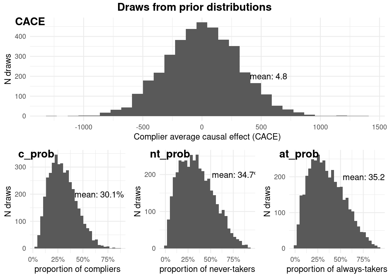

In our example, the prior information assumes the impact of the treatment is centered around zero, with the distributions of compliance types being relatively balanced.

Model fitting and diagnostics

After tailoring prior parameters to reflect our existing knowledge, we proceed with fitting the model. This step combines our prior beliefs with the observed data to update our understanding of the causal effect.

ivobj <- biva$new(
  data = df, y = "Y", d = "D", z = "Z",
  x_ymodel = c("X"),
  x_smodel = c("X"),
  ER = 1,
  side = 2,
  beta_mean_ymodel = cbind(rep(5000, 4), rep(0, 4)),
  beta_sd_ymodel = cbind(rep(200, 4), rep(200, 4)),
  beta_mean_smodel = matrix(0, 2, 2),
  beta_sd_smodel = matrix(1, 2, 2),
  sigma_shape_ymodel = rep(1, 4),
  sigma_scale_ymodel = rep(1, 4),
  fit = TRUE
)

To ensure the model is behaving as expected, we inspect the trace plot of outcomes across different compliance strata. This diagnostic tool helps us confirm satisfactory mixing and convergence of our Markov Chain Monte Carlo (MCMC) sampling process.

ivobj$tracePlot()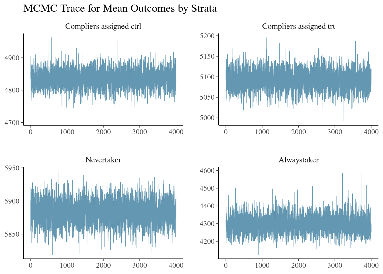

The trace plots show good mixing and convergence, indicating that our MCMC sampler is effectively exploring the posterior distribution. This gives us confidence in the reliability of our posterior estimates.

Next, we conduct a weak instrument test. This is crucial in instrumental variable analysis, as weak instruments can lead to biased estimates and unreliable inferences.

ivobj$weakIVTest()

The instrument is not considered weak, resulting in an estimated 49% of compliers in the population.

The test indicates no cause for concern regarding weak instruments. This means our encouragement (the instrument) is sufficiently correlated with the actual use of the AI translation feature, allowing us to make reliable causal inferences.

How does BIVA tests if you have a weak instrument?

BIVA measures the “strength” of an instrument to be the proportion of compliers. We use an empirical rule-of-thumb of <10% to determine an instrument to be weak, and throw out warnings. A weak instrument case will be discussed later below.

Posterior Summary and Business Insights

Now, we harness the power of Bayesian analysis to extract meaningful insights tailored to our business questions. The BIVA package provides a suite of methods to summarize the findings.

# Posterior distribution of the strata probability
ivobj$strataProbEstimate()

Given the data, we estimate that there is a 49% probability that the unit is a complier, a 42% probability that the unit is a never-taker, and a 10% probability that the unit is an always-taker.

# Posterior probability that CACE is greater than 200
ivobj$calcProb(a = 200)

Given the data, we estimate that the probability that the effect is more than 200 is 95%.

# Posterior median of the CACE
ivobj$pointEstimate()

[1] 257.5321

# Posterior mean of the CACE
ivobj$pointEstimate(median = FALSE)

[1] 257.4584

# 75% credible interval of the CACE
ivobj$credibleInterval()

Given the data, we estimate that there is a 75% probability that the CACE is between 219.54 and 295.89.

# 95% credible interval of the CACE
ivobj$credibleInterval(width = 0.95)

Given the data, we estimate that there is a 95% probability that the CACE is between 190.17 and 323.42.

Through these methods, we obtain precise point estimates, informative probabilistic statements, and a flexible quantification of uncertainty that fuels informed decision-making.

Visualization of Knowledge Progression

The evolution of our understanding, from prior knowledge to the updated posterior informed by data, can be vividly visualized. This visualization is particularly powerful in a business context, as it allows stakeholders to see how our beliefs about the effectiveness of the AI content suggestion tool have changed based on the data we’ve collected.

In our example, we wanted to make a decision based on whether the impact of the tool on watch time is substantial enough to justify its computational costs. Specifically, we set a threshold of 200 hours of increased watch time per week as our decision boundary.

ivobj$vizdraws(
  display_mode_name = TRUE, breaks = 200,
  break_names = c("< 200", "> 200")
)

This approach allows us to answer our business question directly and probabilistically. In this case, we can conclude that there’s strong evidence that the AI content suggestion tool increases watch time by more than 200 hours per week, justifying its computational costs.

Importantly, this method provides a nuanced view that goes beyond simple “significant” or “not significant” dichotomies. It allows decision-makers to weigh the probabilities of different effect sizes against their specific business contexts and risk tolerances.

Binary Outcomes

Let’s explore a scenario that underscores the challenges of causal inference in a real-world product development setting.

Imagine you’re a data scientist at a fast-growing productivity app company. The app offers a free version with basic features and a premium subscription that unlocks a suite of advanced tools. Eager to boost conversions, the product team recently launched a new, interactive in-app tutorial showcasing these premium features and their benefits.

However, the product team launched the tutorial without consulting the impact measurement team beforehand. Now, the tutorial is available to all users.

The impact measurement team, recognizing the need to assess the tutorial’s effectiveness, recommends an “encouragement design.” This involves randomly encouraging a subset of users to complete the tutorial, perhaps through a pop-up notification or a personalized email. Given that anyone, encouraged or not, can use the tutorial, this will be have non compliance in both sides.

The challenge lies in isolating the causal impact of the tutorial, given that it’s already available to everyone. BIVA, by leveraging the random encouragement as an instrument, can estimate the causal effect of the tutorial on premium subscription conversion among compliers - those who will complete the tutorial had they been encouraged, and will not complete the tutorial had they not been encouraged.

Let’s create a simulated dataset that mirrors this situation:

library(dplyr)
library(purrr)
library(broom)

set.seed(2025)
n <- 500

users <- tibble(
  user_id = 1:n,
  X = rpois(n, lambda = 30),
  U = rbinom(n, 1, 0.3)
)

determine_strata <- function(X, U) {
  prob_c <- plogis(-1 + 0.02*X + 2*U)    
  prob_nt <- plogis(-0.5 - 0.01*X - 2*U) 
  prob_at <- 1 - prob_c - prob_nt
  
  sample(c("complier", "never-taker", "always-taker"), 1, 
         prob = c(prob_c, prob_nt, prob_at))
}

users <- users %>%
  mutate(
    strata = map2_chr(X, U, determine_strata),
    Z = rep(c(0, 1), each = n/2),
    D = case_when(
      strata == "always-taker" ~ 1,
      strata == "complier" & Z == 1 ~ 1,
      TRUE ~ 0
    )
  )

generate_outcome <- function(X, U, D, strata) {
  base_prob <- plogis(-2 + 0.03*X + 2*U)  
  
  prob <- case_when(
    strata == "complier" & D == 1 ~ plogis(-2.4 + 0.03*X + 2*U),
    strata == "never-taker" ~ plogis(-2.2 + 0.03*X + 2*U),
    strata == "always-taker" ~ plogis(-1.5 + 0.03*X + 2*U),  
    TRUE ~ base_prob
  )
  
  rbinom(1, 1, prob)
}

users <- users %>%
  rowwise() %>%
  mutate(Y = generate_outcome(X, U, D, strata)) %>%
  ungroup()

# Calculate the true effect for compliers
average_effect <- users %>%
  filter(strata == "complier") %>%
  group_by(Z) %>%
  summarise(mean_y = mean(Y)) %>%
  summarise(difference = mean_y[Z == 1] - mean_y[Z == 0]) %>%
  pull(difference)

print(paste("The average effect of the tutorial on the probability of becoming a premium member for compliers is:", round(average_effect, 4)))

[1] "The average effect of the tutorial on the probability of becoming a premium member for compliers is: -0.0813"

The Pitfall of Naive Analysis

Before we delve into BIVA, let’s see what a naive logistic regression would tell us:

# Naive logistic regression
naive_model <- glm(Y ~ D + X, data = users, family = binomial)

# Display results
tidy(naive_model, conf.int = T) %>%
  mutate(p.value = format.pval(p.value, eps = 0.001)) %>%
  knitr::kable(digits = 3)

term	estimate	std.error	statistic	p.value	conf.low	conf.high
(Intercept)	-1.191	0.554	-2.151	0.031471	-2.287	-0.113
D	0.337	0.185	1.823	0.068291	-0.025	0.701
X	0.018	0.018	1.023	0.306368	-0.017	0.053

This naive analysis suggests that completing the tutorial is associated with an increased likelihood of premium conversion. It’s a tempting conclusion, but it’s also likely because it fails to account for selection bias. Users predisposed to premium conversion might also be more likely to complete the tutorial, creating a spurious positive association.

In reality, our data generating process is such that the tutorial actually has a negative effect on conversion for compliers. This stark discrepancy underscores the critical importance of proper causal inference techniques like instrumental variables analysis. Without them, we risk not just misunderstanding our data, but making counterproductive business decisions.

Prior predictive checking

The outcome type is specified by having y_type = “binary”. We assume exclusion restriction, so ER = 1. With two-side noncompliance, we set side = 2. The parameters in the prior distributions are specified as well. We first look into what the prior distributions assume about the parameters.

ivobj <- biva::biva$new(
  data = users, 
  y = "Y", d = "D", z = "Z",
  x_ymodel = c("X"),
  x_smodel = c("X"),
  y_type = "binary",
  ER = 1,
  side = 2,
  beta_mean_ymodel = matrix(0, 4, 2),
  beta_sd_ymodel = matrix(0.05, 4, 2),
  beta_mean_smodel = matrix(0, 2, 2),
  beta_sd_smodel = matrix(0.1, 2, 2),
  fit = FALSE
)

ivobj$plotPrior()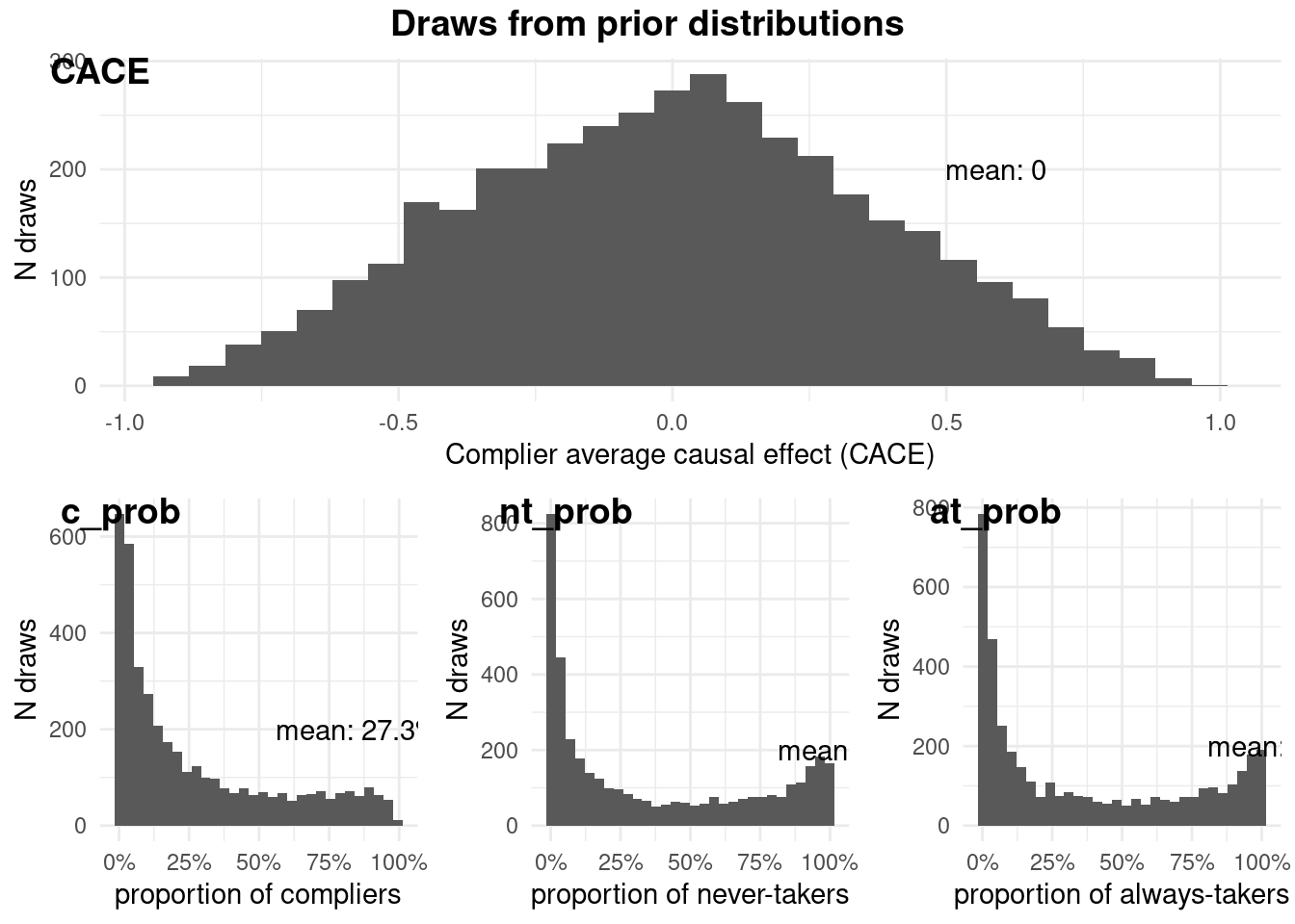

These prior distributions reflect our initial beliefs about the parameters. They’re intentionally weak, but not compleatly uniformative. For example, they refect that a small CACE is more likely than a big one. The plots show the range of plausible values for each parameter before we’ve seen any data.

Fitting a BIVA model to the data

Now we fit a BIVA model to the data.

ivobj <- biva::biva$new(
  data = users,
  y = "Y", d = "D", z = "Z",
  x_ymodel = c("X"),
  x_smodel = c("X"),
  y_type = "binary",
  ER = 1,
  side = 2,
  beta_mean_ymodel = matrix(0, 4, 2),
  beta_sd_ymodel = matrix(0.05, 4, 2),
  beta_mean_smodel = matrix(0, 2, 2),
  beta_sd_smodel = matrix(0.1, 2, 2),
  fit = TRUE
)

Fitting model to the data

All diagnostics look fine

We look at the trace plot of outcomes in each strata. The four plots are the posterior draws of the mean outcomes among the compliers assinged to control, the compliers nudged to treatment, the never-takers, and the always-takers.

ivobj$tracePlot()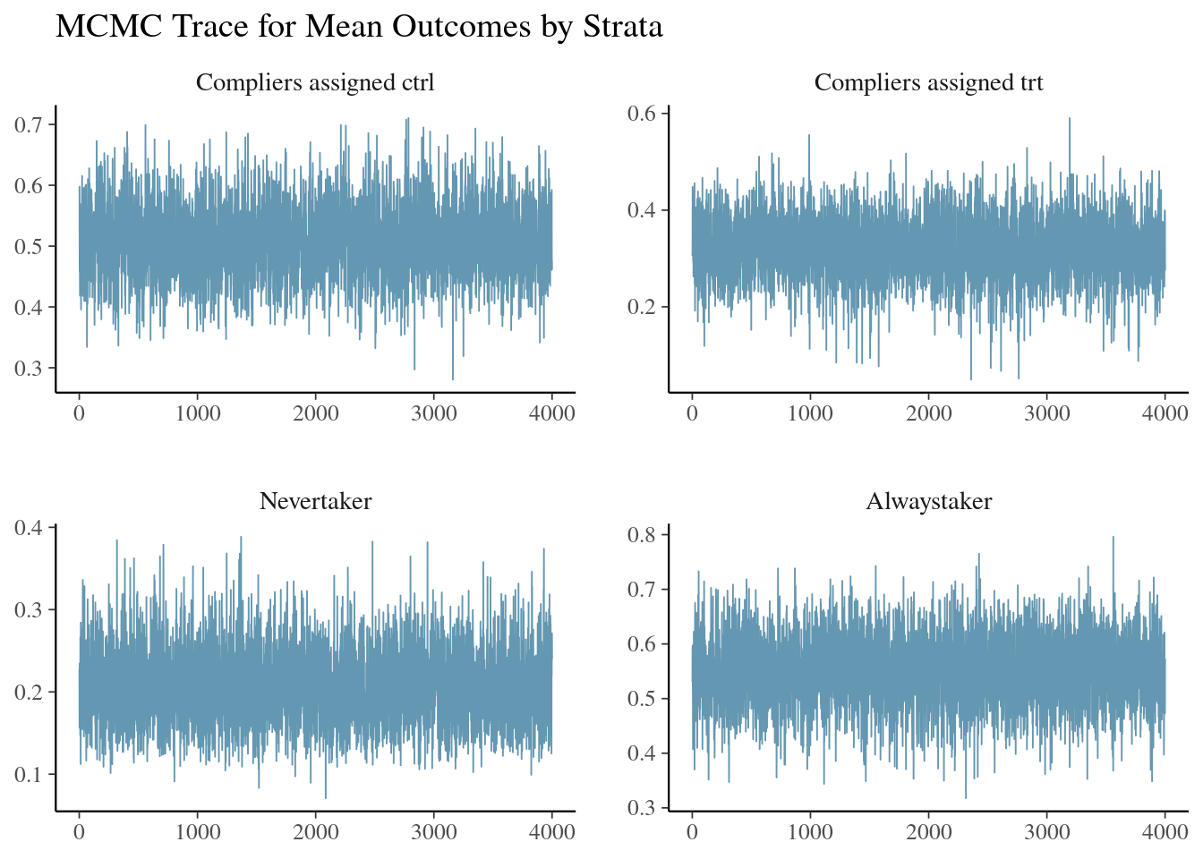

The convergence and mixing look good.

We run the weak instrument test.

ivobj$weakIVTest()

The instrument is not considered weak, resulting in an estimated 50% of compliers in the population.

No weak instrument issue is detected.

Now for the million-dollar question: Does completing the tutorial increase the likelihood of premium subscriptions? Let’s visualize how our priors get updated after analyzing the data with BIVA:

ivobj$vizdraws(
  display_mode_name = TRUE
)

The results are striking. BIVA correctly reveals the tutorial’s negative impact on conversion rates among compliers, a crucial insight that the naive approach missed entirely. This demonstrates the power of proper causal inference in uncovering counter-intuitive truths hidden in our data.

In the world of product development, such insights are gold. They prevent us from doubling down on ineffective strategies and guide us toward truly impactful improvements. This case study serves as a potent reminder: in the quest for causality, your choice of analytical tool can make all the difference between misleading conclusions and actionable insights.

Caveat 1: Generic Mixing Issue

On the technical side, Bayesian analysis relies on posterior sampling for estimating the distributions of parameters that we get from the above methods. Mixing is a term that measures whether the sampling process is stabilized yet. Ideally, we want good mixing behavior from the posterior distribution that tells us “results are ready for interpretation!” If that does not happen, we should reserve the right to be informed of any mixing issue so we will be able to decide if there is anything we could do to help, or there is not much we can do so we interpret the results with caution.

The trace plot analysis in the BIVA workflow enables us to take such responsibility. After fitting the model, the trace plot analysis should follow immediately. This happens prior to summarizing and interpreting the results from posterior so the users are not committting any crimes of “hacking” anything. Instead, it is a responsible practice of understanding how you end up with the results and whether there could any issue with their validity that invites fixes or caution. We used the same setting of the AI feature example above for illustration, but the data are generated from a difference seed.

set.seed(2001)  # Set random seed for reproducibility
n <- 200         # Total number of individuals

# Generate Covariates:
# X: Continuous, observed covariate
X <- rnorm(n)      # Draw from standard normal distribution

# U: Binary, unobserved confounder
U <- rbinom(n, 1, 0.5)  # 1 = U = 1 with 50% probability

# Determine True Principal Strata (PS) Membership:
# 1: Complier, 2: Never-taker, 3: Always-taker
true.PS <- rep(0, n)       # Initialize PS vector
U1.ind <- (U == 1)       # Indices where U = 1
U0.ind <- (U == 0)       # Indices where U = 0
num.U1 <- sum(U1.ind)    # Number of individuals with U = 1
num.U0 <- sum(U0.ind)    # Number of individuals with U = 0

# Assign PS membership based on U:
# For U = 1: 60% compliers, 30% never-takers, 10% always-takers
# For U = 0: 40% compliers, 50% never-takers, 10% always-takers
true.PS[U1.ind] <- t(rmultinom(num.U1, 1, c(0.6, 0.3, 0.1))) %*% c(1, 2, 3)
true.PS[U0.ind] <- t(rmultinom(num.U0, 1, c(0.4, 0.5, 0.1))) %*% c(1, 2, 3)

# Assign Treatment (Z):
# Half the individuals are assigned to treatment (Z = 1), half to control (Z = 0)
Z <- c(rep(0, n / 2), rep(1, n / 2))

# Determine Treatment Received (D) Based on PS and Z:
D <- rep(0, n)            # Initialize treatment received vector

# Define indices for each group:
c.trt.ind <- (true.PS == 1) & (Z == 1)  # Compliers, treatment
c.ctrl.ind <- (true.PS == 1) & (Z == 0)  # Compliers, control
nt.ind <- (true.PS == 2)               # Never-takers
at.ind <- (true.PS == 3)               # Always-takers

# Count individuals in each group:
num.c.trt <- sum(c.trt.ind)
num.c.ctrl <- sum(c.ctrl.ind)
num.nt <- sum(nt.ind)
num.at <- sum(at.ind)

# Assign treatment received:
D[at.ind] <- rep(1, num.at)   # Always-takers receive treatment
D[c.trt.ind] <- rep(1, num.c.trt) # Compliers in treatment group receive treatment

# Generate Observed Outcome (Y):
Y <- rep(0, n) # Initialize outcome vector

# Outcome model for compliers in control group:
Y[c.ctrl.ind] <- rnorm(num.c.ctrl,
 mean = 5000 + 100 * X[c.ctrl.ind] - 300 * U[c.ctrl.ind],
 sd = 50
)

# Outcome model for compliers in treatment group:
Y[c.trt.ind] <- rnorm(num.c.trt,
 mean = 5250 + 100 * X[c.trt.ind] - 300 * U[c.trt.ind],
 sd = 50
)

# Outcome model for never-takers:
Y[nt.ind] <- rnorm(num.nt,
 mean = 6000 + 100 * X[nt.ind] - 300 * U[nt.ind],
 sd = 50
)

# Outcome model for always-takers:
Y[at.ind] <- rnorm(num.at,
 mean = 4500 + 100 * X[at.ind] - 300 * U[at.ind],
 sd = 50
)

# Create a data frame with all variables:
df <- data.frame(Y = Y, Z = Z, D = D, X = X, U = U)

Model fitting and diagnostics

Now that we inherit the above setting and assumptions, we cut to the chase of fitting the model and running diagnostics.

ivobj <- biva$new(
  data = df, y = "Y", d = "D", z = "Z",
  x_ymodel = c("X"),
  x_smodel = c("X"),
  ER = 1,
  side = 2,
  beta_mean_ymodel = cbind(rep(5000, 4), rep(0, 4)),
  beta_sd_ymodel = cbind(rep(200, 4), rep(200, 4)),
  beta_mean_smodel = matrix(0, 2, 2),
  beta_sd_smodel = matrix(1, 2, 2),
  sigma_shape_ymodel = rep(1, 4),
  sigma_scale_ymodel = rep(1, 4),
  fit = TRUE
)

Warning: The largest R-hat is 1.53, indicating chains have not mixed.
Running the chains for more iterations may help. See
https://mc-stan.org/misc/warnings.html#r-hat

Warning: Bulk Effective Samples Size (ESS) is too low, indicating posterior means and medians may be unreliable.
Running the chains for more iterations may help. See
https://mc-stan.org/misc/warnings.html#bulk-ess

Warning: Tail Effective Samples Size (ESS) is too low, indicating posterior variances and tail quantiles may be unreliable.
Running the chains for more iterations may help. See
https://mc-stan.org/misc/warnings.html#tail-ess

Warning in initialize(...): Only 50% of the Rhats are less than 1.1Only 50% of
n_eff/N are greater than 0.001Only 50% of n_eff are greater than 100

We already see some warning messages automatically returned by methods in the pakcage. The following diagnostic tool will give us the trace plot for a visualization of any issue with mixing and convergence.

ivobj$tracePlot()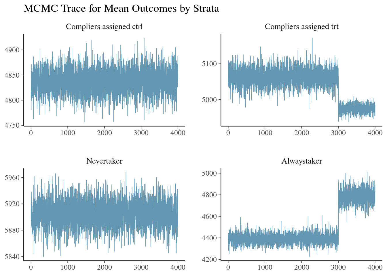

The mixing behavior is not ideal. The posterior samples of outcomes among nudged compliers and always-takers wandered through some regions that they did not later explore. The poor mixing issue is discovered.

Like a doctor precribing more tests when they first find out some symptoms, we run the weak instrument test below to make sure the analysis is not suffering from a more severe systematic disease.

ivobj$weakIVTest()

The instrument is not considered weak, resulting in an estimated 47% of compliers in the population.

Luckily, the poor mixing issue is not caused and compounded by a weak instrument issue. It is a relatively generic mixing issue. Without the aid of more information, nudged compliers can be confused with always-takers since they will both be observed to adopt the AI feature if nudged.

Here are some possible fixes by our recommended order.

1. More data: Data are information. A larger sample size can resolve a lot of nonsystematic issues that are masked or unclear in a small sample.
2. Knowledge through prior: Even though we recommend users to input prior parameters that best reflect their prior knowledge in the first stage, the mixing issue calls for a second round of reflection to reaffirm that the input represent the best efforts of reporting our knowledge.
3. Generic fixes: Common practice of increasing the number of iterations, or running them more slowly could be tried out.

The order of fixes suggests prioritizing understanding what went wrong in terms of inadequate amount or quality of information through data and models, instead of jumping into instant investment of time and resources on generic solutions.

After the step of brainstorming and implementing solutions, if the mixing issue persists, the results from the analysis can still be valuable when interpreted with caution.

Posterior Summary and Business Insights

Assume we did not go with any fixes that change the data or model, we will still be able to get the results.

# Posterior distribution of the strata probability
ivobj$strataProbEstimate()

Given the data, we estimate that there is a 47% probability that the unit is a complier, a 38% probability that the unit is a never-taker, and a 15% probability that the unit is an always-taker.

# Posterior probability that CACE is greater than 200
ivobj$calcProb(a = 200)

Given the data, we estimate that the probability that the effect is more than 200 is 60%.

# Posterior median of the CACE
ivobj$pointEstimate()

[1] 213.2548

# Posterior mean of the CACE
ivobj$pointEstimate(median = FALSE)

[1] 203.6615

# 75% credible interval of the CACE
ivobj$credibleInterval()

Given the data, we estimate that there is a 75% probability that the CACE is between 133.62 and 256.6.

# 95% credible interval of the CACE
ivobj$credibleInterval(width = 0.95)

Given the data, we estimate that there is a 95% probability that the CACE is between 103.98 and 282.99.

The point estimates become less accurate compared to the case when we do not have mixing issue, and the credible intervals become wider. A larger amount of uncertainty is the consequence of poor mixing. It reminds us to be less reliant on the point estimates in this case. Credible intervals and posterior probability are good measures for us to summarize that we still anticipate a positive effect of the AI feature but there is the amount of uncertainty measured by the range or the probability we report.

Visualization of Knowledge Progression

The visualization tool in our package is another good way of discerning the mixing issue and its implication on impact measurement. We will notice a bimodal posterior distribution, and understand that more uncertainty origins from the two modes.

ivobj$vizdraws(
  display_mode_name = TRUE, breaks = 200,
  break_names = c("< 200", "> 200")
)

Caveat 2: Weak Instrument Issue

We measure the “strength” of an instrumental variable to be the proportion of compliers in the entire population. Weak instrument issue is a more serious systematic issue that deprives the RED and IV analysis of their magic. It can incur many issues:

1. Difficulty in predicting the imbalanced compliance types, and thus the CACE
2. Little information in data to update the prior knowledge on the impact
3. Sensitivity to priors
4. Unreliable point estimate
5. Wide credible intervals

The interpretation of the impact measurement will also be limited to a small proportion of units in the entire population.

We use a different data generating process for the AI feature example where the proportion of compliers to the nudge is only arount 5% of the population.

set.seed(1997)    # Set random seed for reproducibility
n <- 1000         # Total number of individuals

# Generate Covariates:
# X: Continuous, observed covariate
X <- rnorm(n)      # Draw from standard normal distribution

# U: Binary, unobserved confounder
U <- rbinom(n, 1, 0.5)  # 1 = U = 1 with 50% probability

# Determine True Principal Strata (PS) Membership:
# 1: Complier, 2: Never-taker, 3: Always-taker
true.PS <- rep(0, n)       # Initialize PS vector
U1.ind <- (U == 1)       # Indices where U = 1
U0.ind <- (U == 0)       # Indices where U = 0
num.U1 <- sum(U1.ind)    # Number of individuals with U = 1
num.U0 <- sum(U0.ind)    # Number of individuals with U = 0

# Assign PS membership based on U:
# For U = 1: 6% compliers, 70% never-takers, 24% always-takers
# For U = 0: 4% compliers, 70% never-takers, 26% always-takers
true.PS[U1.ind] <- t(rmultinom(num.U1, 1, c(0.06, 0.7, 0.24))) %*% c(1, 2, 3)
true.PS[U0.ind] <- t(rmultinom(num.U0, 1, c(0.04, 0.7, 0.26))) %*% c(1, 2, 3)

# Assign Treatment (Z):
# Half the individuals are assigned to treatment (Z = 1), half to control (Z = 0)
Z <- c(rep(0, n / 2), rep(1, n / 2))

# Determine Treatment Received (D) Based on PS and Z:
D <- rep(0, n)            # Initialize treatment received vector

# Define indices for each group:
c.trt.ind <- (true.PS == 1) & (Z == 1)  # Compliers, treatment
c.ctrl.ind <- (true.PS == 1) & (Z == 0)  # Compliers, control
nt.ind <- (true.PS == 2)               # Never-takers
at.ind <- (true.PS == 3)               # Always-takers

# Count individuals in each group:
num.c.trt <- sum(c.trt.ind)
num.c.ctrl <- sum(c.ctrl.ind)
num.nt <- sum(nt.ind)
num.at <- sum(at.ind)

# Assign treatment received:
D[at.ind] <- rep(1, num.at)   # Always-takers receive treatment
D[c.trt.ind] <- rep(1, num.c.trt) # Compliers in treatment group receive treatment

# Generate Observed Outcome (Y):
Y <- rep(0, n) # Initialize outcome vector

# Outcome model for compliers in control group:
Y[c.ctrl.ind] <- rnorm(num.c.ctrl,
 mean = 5000 + 100 * X[c.ctrl.ind] - 300 * U[c.ctrl.ind],
 sd = 50
)

# Outcome model for compliers in treatment group:
Y[c.trt.ind] <- rnorm(num.c.trt,
 mean = 5250 + 100 * X[c.trt.ind] - 300 * U[c.trt.ind],
 sd = 50
)

# Outcome model for never-takers:
Y[nt.ind] <- rnorm(num.nt,
 mean = 6000 + 100 * X[nt.ind] - 300 * U[nt.ind],
 sd = 50
)

# Outcome model for always-takers:
Y[at.ind] <- rnorm(num.at,
 mean = 4500 + 100 * X[at.ind] - 300 * U[at.ind],
 sd = 50
)

# Create a data frame with all variables:
df <- data.frame(Y = Y, Z = Z, D = D, X = X, U = U)

Model fitting and diagnostics

We jump to model fitting and diagnostics.

ivobj <- biva$new(
  data = df, y = "Y", d = "D", z = "Z",
  x_ymodel = c("X"),
  x_smodel = c("X"),
  ER = 1,
  side = 2,
  beta_mean_ymodel = cbind(rep(5000, 4), rep(0, 4)),
  beta_sd_ymodel = cbind(rep(200, 4), rep(200, 4)),
  beta_mean_smodel = matrix(0, 2, 2),
  beta_sd_smodel = matrix(1, 2, 2),
  sigma_shape_ymodel = rep(1, 4),
  sigma_scale_ymodel = rep(1, 4),
  fit = TRUE
)

Warning: The largest R-hat is 1.53, indicating chains have not mixed.
Running the chains for more iterations may help. See
https://mc-stan.org/misc/warnings.html#r-hat

Warning: Bulk Effective Samples Size (ESS) is too low, indicating posterior means and medians may be unreliable.
Running the chains for more iterations may help. See
https://mc-stan.org/misc/warnings.html#bulk-ess

Warning: Tail Effective Samples Size (ESS) is too low, indicating posterior variances and tail quantiles may be unreliable.
Running the chains for more iterations may help. See
https://mc-stan.org/misc/warnings.html#tail-ess

Warning in initialize(...): Only 50% of the Rhats are less than 1.1Only 50% of
n_eff/N are greater than 0.001Only 50% of n_eff are greater than 100

We run the diagnostic tools.

ivobj$tracePlot()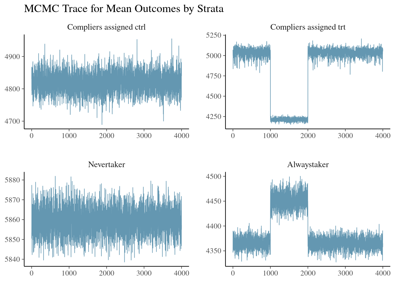

We detect a mixing issue again.

ivobj$weakIVTest()

The instrument is considered weak, resulting in an estimated 6% of compliers in the population. Posterior point estimates of the CACE might be unreliable.

This time the mixing issue is compounded by a weak instrument issue.

We could still try the fixes suggested for the generic mixing issue. However, a weak instrument issue is really detrimental to the analysis in the sense that none of the fixes could really drastically improve the quality of the analysis even if we have a large sample size. Therefore, during the study design phase, it is important to have a devised RED with a nudge attractive enough to induce a high proportion of compliers. If that does not happen, during the analysis phase, we recommend that users proceed to truthfully present the findings from the posterior summary and quantify the uncertainty in the impact measurement through credible interval or posterior probability. Posterior point estimates can be unreliable in this weak instrument case.

Posterior Summary and Business Insights

We display the results for us to better understand the consequences of a weak IV issue.

# Posterior distribution of the strata probability
ivobj$strataProbEstimate()

Given the data, we estimate that there is a 6% probability that the unit is a complier, a 68% probability that the unit is a never-taker, and a 26% probability that the unit is an always-taker.

# Posterior probability that CACE is greater than 200
ivobj$calcProb(a = 200)

Given the data, we estimate that the probability that the effect is more than 200 is 50%.

# Posterior median of the CACE
ivobj$pointEstimate()

[1] 200.1115

# Posterior mean of the CACE
ivobj$pointEstimate(median = FALSE)

[1] 13.64431

# 75% credible interval of the CACE
ivobj$credibleInterval()

Given the data, we estimate that there is a 75% probability that the CACE is between -601.19 and 267.62.

# 95% credible interval of the CACE
ivobj$credibleInterval(width = 0.95)

Given the data, we estimate that there is a 95% probability that the CACE is between -640.23 and 308.01.

The point estimate by the posterior mean is way off, but the posterior median is relatively robust. The credible intervals are too wide to be informative.

Visualization of Knowledge Progression

The visualization tool shows that the two modes are completely separated, which explains why the credible interval ranges from large negative values to large positive values.

ivobj$vizdraws(
  display_mode_name = TRUE, breaks = 200,
  break_names = c("< 200", "> 200")
)

Further Exploration

To delve deeper into the intricacies of instrumental variable analysis and causal inference, we recommend the following resources:

• McElreath (2018) Statistical Rethinking: Instruments and causal designs.
• Angrist, Imbens, and Rubin (1996) Identification of causal effects using instrumental variables.
• Frangakis and Rubin (2002) Principal stratification in causal inference.
• G. Imbens (2014) Instrumental variables: An econometrician’s perspective.
• G. W. Imbens and Rubin (1997) Bayesian inference for causal effects in randomized experiments with noncompliance.
• Liu and Li (2023) PStrata: An R Package for Principal Stratification.
• VanderWeele (2011) Principal stratification–uses and limitations.
• Li (2022) Post-treatment confounding: Principal Stratification.

Angrist, Joshua D, Guido W Imbens, and Donald B Rubin. 1996. “Identification of Causal Effects Using Instrumental Variables.” Journal of the American Statistical Association 91 (434): 444–55. https://doi.org/10.1080/01621459.1996.10476902.

Frangakis, Constantine E, and Donald B Rubin. 2002. “Principal Stratification in Causal Inference.” Biometrics 58 (1): 21–29. https://doi.org/10.1111/j.0006-341X.2002.00021.x.

Imbens, Guido. 2014. “Instrumental Variables: An Econometrician’s Perspective.” National Bureau of Economic Research. https://doi.org/10.3386/w19983.

Imbens, Guido W., and Donald B. Rubin. 1997. “Bayesian Inference for Causal Effects in Randomized Experiments with Noncompliance.” The Annals of Statistics 25 (1): 305–27. http://www.jstor.org/stable/2242722.

Li, Fan. 2022. “STA 640 — Causal Inference Unit 6.2: Post-Treatment Confounding: Principal Stratification.” https://www2.stat.duke.edu/~fl35/teaching/640/Chapter6.2_principal%20stratification.pdf.

Liu, Bo, and Fan Li. 2023. “PStrata: An r Package for Principal Stratification.” https://arxiv.org/abs/2304.02740.

McElreath, R. 2018. Statistical Rethinking: A Bayesian Course with Examples in r and Stan. Chapman &Amp; Hall/CRC Texts in Statistical Science. CRC Press. https://books.google.com/books?id=T3FQDwAAQBAJ.

VanderWeele, Tyler J. 2011. “Principal Stratification–Uses and Limitations.” The International Journal of Biostatistics 7 (1): 0000102202155746791329. https://doi.org/10.2202/1557-4679.1329.