8 The Power of Randomization

It is crucial to recognize that randomization isn’t magic. When a sufficiently large population is randomly divided into two groups, these groups will be remarkably similar in both observable and unobservable characteristics. By assigning one group to a treatment and leaving the other as a control, any difference in the outcome of interest can be confidently attributed to the treatment. As we discussed in Chapter 1, causal inference can be conceptualized as a missing data problem. In a randomized experiment, this problem is simplified because we effectively have data missing at random, allowing us to make unbiased estimates of causal effects.

8.1 The Importance of SUTVA: The Cornerstone of Valid Inference

However, it’s crucial to remember that the success of both RCTs and A/B tests hinges on a fundamental assumption: the Stable Unit Treatment Value Assumption (SUTVA). SUTVA has two main components:

No Interference (or No Spillover): The treatment applied to one unit should not affect the outcome of another unit. This means that the outcome for any unit is unaffected by the treatments received by other units.
Treatment Variation Irrelevance (or Consistency): The potential outcome of a unit under a specific treatment should be the same regardless of how that treatment is assigned. This implies that if a unit receives a particular treatment, the outcome should only depend on that treatment, not on how or why it was assigned.

In simpler terms, SUTVA ensures that the effect of the treatment is solely due to the treatment itself and not influenced by other factors or interactions between units.

SUTVA Violations: When the Ideal Meets Reality

While SUTVA is often assumed, it can be easily violated:

Network Effects: Consider an A/B test of a new social media feature. If users in the treatment group interact with users in the control group, the feature’s impact might spread beyond the intended group, violating SUTVA.
Market Competition: Testing a new pricing strategy might trigger competitor reactions, indirectly affecting the outcome even for users not exposed to the new price.
Spillover Effects: In advertising, a targeted campaign for one product might unintentionally increase awareness or sales of related products.

Mitigating SUTVA Violations

Sometimes, the solution to a SUTVA violation can be as simple as changing the unit of randomization. For instance, running geo-experiments in geographically isolated markets can minimize interaction between groups. In other cases, solutions require more intricate study designs. When complete elimination isn’t feasible, it’s crucial to acknowledge and mitigate the potential impact of SUTVA violations on your conclusions.

Key Takeaway:

Understanding and addressing SUTVA is essential for designing experiments and drawing valid conclusions. By carefully considering the potential for interference and inconsistency, researchers and practitioners can design more robust experiments and make more informed decisions based on their findings.

8.2 An example using code

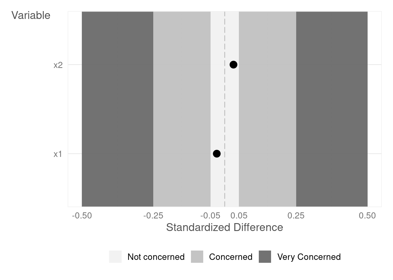
The {imt} package provides a convenient way to randomize while ensuring baseline equivalence. The imt::randomize function iteratively re-randomizes until achieving a specified level of baseline equivalence (see Section 3.1) or reaching a maximum number of attempts.

my_data <- tibble::tibble(
  x1 = rnorm(10000), 
  x2 = rnorm(10000)
)

# Randomize
randomized <- imt::randomizer$new(
  data = my_data, 
  seed = 12345, 
  max_attempts = 1000,
  variables = c("x1", "x2"), 
  standard = "Not Concerned"
)

# Get Randomized Data
randomized$data

# A tibble: 10,000 × 3
       x1      x2 treated
    <dbl>   <dbl> <lgl>  
 1 -0.370  0.747  TRUE   
 2 -0.456 -1.86   TRUE   
 3  1.73   0.494  TRUE   
 4  0.565  0.346  TRUE   
 5 -0.432 -0.671  FALSE  
 6 -1.56  -0.462  FALSE  
 7 -0.368 -1.09   FALSE  
 8  0.693 -0.0533 TRUE   
 9 -1.48   0.740  TRUE   
10  1.38  -0.0855 TRUE   
# ℹ 9,990 more rows

# Get Balance Summary
randomized$balance_summary

# A tibble: 2 × 3
  variables std_diff balance      
  <chr>        <dbl> <fct>        
1 x1         -0.0278 Not Concerned
2 x2          0.0307 Not Concerned

# Generate Balance Plot
randomized$balance_plot

8.3 Stratified Randomization

While random assignment is effective, unforeseen factors can sometimes lead to imbalanced groups. Stratified randomization addresses this by dividing users into subgroups (strata) based on relevant characteristics that are believed to influence the outcome metric. Randomization is then performed within each stratum, ensuring that both treatment and control groups have a similar proportion of users from each subgroup.

This approach strengthens experiments by creating balanced groups. For instance, if user location is expected to affect the outcome metric, users can be stratified by location (e.g., urban vs. rural), followed by randomization within each location. This ensures a similar distribution of user attributes across treatment and control groups, controlling for confounding factors—user traits that impact both exposure to the new feature and the desired outcome. With balanced groups, any observed differences in the outcome metric are more likely due to the new feature itself, leading to more precise and reliable results.

Examples

Targeting Mobile App Engagement: In an RCT to evaluate a new in-app notification, user location (urban vs. rural) is suspected to influence user response. Stratification by location, followed by randomization within each stratum, can control for this factor.
Personalizing a Recommendation Engine: When A/B testing a revamped recommendation engine, past purchase history is hypothesized to influence user response. Stratification by purchase history categories (e.g., frequent buyers of clothing vs. electronics), followed by randomization within each category, can account for this.

Advantages:

Reduced bias: Stratification helps isolate the true effect of the new feature by controlling for the influence of confounding factors. This leads to more reliable conclusions about the feature’s impact on user behavior.
Improved decision-making: By pinpointing the feature’s effect on specific user groups (e.g., urban vs. rural in the notification example), stratified randomization can inform decisions about targeted rollouts or further iterations based on subgroup performance.

Disadvantages:

Increased complexity: Designing and implementing stratified randomization requires careful planning to choose the right stratification factors and ensure enough users within each stratum for valid analysis.
Need for larger sample sizes: Maintaining balance across strata might necessitate a larger overall sample size compared to simple random assignment.

Example with code

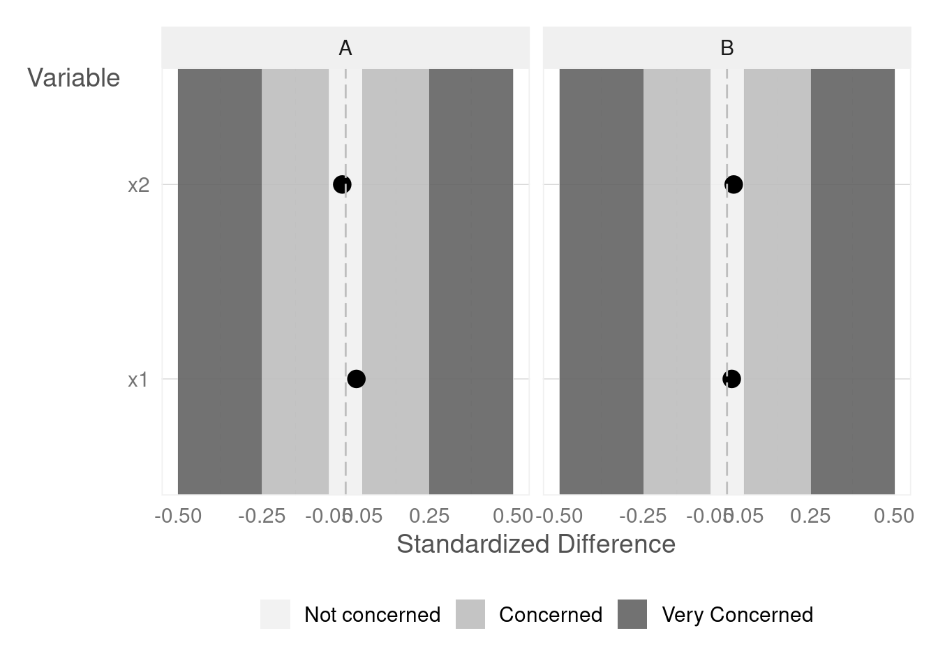
Let’s illustrate the concept of stratified randomization with a practical example. Consider a scenario where we have data on 10,000 individuals, each described by two continuous variables (x1 and x2) and two categorical variables (x3 and x4). We suspect that variable x3 might be a confounding factor influencing the outcome of our experiment.

my_data <- tibble::tibble(
  x1 = rnorm(10000), 
  x2 = rnorm(10000),
  x3 = rep(c("A", "B"), 5000),
  x4 = rep(c("C", "D"), 5000)
)

# Create a Randomizer Object
randomized <- imt::randomizer$new(
  data = my_data, 
  seed = 12345, 
  max_attempts = 1000,
  variables = c("x1", "x2"), 
  standard = "Not Concerned",
  group_by = "x3"
)

# Generate Balance Plot
randomized$balance_plot

In this code, we’re using the imt::randomizer function to create an object that will help us perform stratified randomization. We specify x3 as the variable to stratify by, ensuring that the treatment and control groups have a balanced distribution of individuals from both categories of x3.

By incorporating stratified randomization into our experimental design, we can effectively control for the influence of variable x3, enhancing the internal validity of our study and allowing for more precise estimates of causal effects.

In conclusion, stratified randomization offers a powerful way to enhance the rigor and precision of experiments, particularly when dealing with potential confounding factors. While it may introduce some additional complexity and potentially require larger sample sizes, the benefits in terms of internal validity and the ability to draw more nuanced conclusions often outweigh these drawbacks. The thoughtful use of stratified randomization can be a valuable asset in the causal inference toolkit.

Learn more

Chernozhukov et al. (2024) Applied causal inference powered by ML and AI.

--- title: "The Power of Randomization" share: permalink: "https://book.martinez.fyi/rct_basic.html" description: "Business Data Science: What Does it Mean to Be Data-Driven?" linkedin: true email: true mastodon: true --- ![Randomization](img/randomization.png){.lightbox} It is crucial to recognize that randomization isn't magic. When a sufficiently large population is randomly divided into two groups, these groups will be remarkably similar in both observable and unobservable characteristics. By assigning one group to a treatment and leaving the other as a control, any difference in the outcome of interest can be confidently attributed to the treatment. As we discussed in Chapter 1, causal inference can be conceptualized as a missing data problem. In a randomized experiment, this problem is simplified because we effectively have data missing at random, allowing us to make unbiased estimates of causal effects. ## The Importance of SUTVA: The Cornerstone of Valid Inference However, it's crucial to remember that the success of both RCTs and A/B tests hinges on a fundamental assumption: the Stable Unit Treatment Value Assumption (SUTVA). SUTVA has two main components: - **No Interference (or No Spillover):** The treatment applied to one unit should not affect the outcome of another unit. This means that the outcome for any unit is unaffected by the treatments received by other units. - **Treatment Variation Irrelevance (or Consistency):** The potential outcome of a unit under a specific treatment should be the same regardless of how that treatment is assigned. This implies that if a unit receives a particular treatment, the outcome should only depend on that treatment, not on how or why it was assigned. In simpler terms, SUTVA ensures that the effect of the treatment is solely due to the treatment itself and not influenced by other factors or interactions between units. #### SUTVA Violations: When the Ideal Meets Reality While SUTVA is often assumed, it can be easily violated: - **Network Effects:** Consider an A/B test of a new social media feature. If users in the treatment group interact with users in the control group, the feature's impact might spread beyond the intended group, violating SUTVA. - **Market Competition:** Testing a new pricing strategy might trigger competitor reactions, indirectly affecting the outcome even for users not exposed to the new price. - **Spillover Effects:** In advertising, a targeted campaign for one product might unintentionally increase awareness or sales of related products. #### Mitigating SUTVA Violations Sometimes, the solution to a SUTVA violation can be as simple as **changing the unit of randomization.** For instance, running geo-experiments in geographically isolated markets can minimize interaction between groups. In other cases, solutions require more intricate study designs. When complete elimination isn't feasible, it's crucial to **acknowledge and mitigate** the potential impact of SUTVA violations on your conclusions. ::: {.callout-note title="Key Takeaway:"} Understanding and addressing SUTVA is essential for designing experiments and drawing valid conclusions. By carefully considering the potential for interference and inconsistency, researchers and practitioners can design more robust experiments and make more informed decisions based on their findings. ::: ## An example using code <img src="https://github.com/google/imt/blob/main/man/figures/logo.png?raw=true" align="right" height="138" alt="" /> The [{imt}](https://github.com/google/imt) package provides a convenient way to randomize while ensuring baseline equivalence. The `imt::randomize` function iteratively re-randomizes until achieving a specified level of baseline equivalence (see @sec-baseline) or reaching a maximum number of attempts. ```{r imt::randomizer} my_data <- tibble::tibble( x1 = rnorm(10000), x2 = rnorm(10000) ) # Randomize randomized <- imt::randomizer$new( data = my_data, seed = 12345, max_attempts = 1000, variables = c("x1", "x2"), standard = "Not Concerned" ) # Get Randomized Data randomized$data # Get Balance Summary randomized$balance_summary # Generate Balance Plot randomized$balance_plot ``` ## Stratified Randomization While random assignment is effective, unforeseen factors can sometimes lead to imbalanced groups. Stratified randomization addresses this by dividing users into subgroups (strata) based on relevant characteristics that are believed to influence the outcome metric. Randomization is then performed within each stratum, ensuring that both treatment and control groups have a similar proportion of users from each subgroup. This approach strengthens experiments by creating balanced groups. For instance, if user location is expected to affect the outcome metric, users can be stratified by location (e.g., urban vs. rural), followed by randomization within each location. This ensures a similar distribution of user attributes across treatment and control groups, controlling for confounding factors—user traits that impact both exposure to the new feature and the desired outcome. With balanced groups, any observed differences in the outcome metric are more likely due to the new feature itself, leading to more precise and reliable results. ### Examples - **Targeting Mobile App Engagement:** In an RCT to evaluate a new in-app notification, user location (urban vs. rural) is suspected to influence user response. Stratification by location, followed by randomization within each stratum, can control for this factor. - **Personalizing a Recommendation Engine:** When A/B testing a revamped recommendation engine, past purchase history is hypothesized to influence user response. Stratification by purchase history categories (e.g., frequent buyers of clothing vs. electronics), followed by randomization within each category, can account for this. ### Advantages: - **Reduced bias:** Stratification helps isolate the true effect of the new feature by controlling for the influence of confounding factors. This leads to more reliable conclusions about the feature's impact on user behavior. - **Improved decision-making:** By pinpointing the feature's effect on specific user groups (e.g., urban vs. rural in the notification example), stratified randomization can inform decisions about targeted rollouts or further iterations based on subgroup performance. ### Disadvantages: - **Increased complexity:** Designing and implementing stratified randomization requires careful planning to choose the right stratification factors and ensure enough users within each stratum for valid analysis. - **Need for larger sample sizes:** Maintaining balance across strata might necessitate a larger overall sample size compared to simple random assignment. ### Example with code Let's illustrate the concept of stratified randomization with a practical example. Consider a scenario where we have data on 10,000 individuals, each described by two continuous variables (x1 and x2) and two categorical variables (x3 and x4). We suspect that variable x3 might be a confounding factor influencing the outcome of our experiment. ```{r stratified} my_data <- tibble::tibble( x1 = rnorm(10000), x2 = rnorm(10000), x3 = rep(c("A", "B"), 5000), x4 = rep(c("C", "D"), 5000) ) # Create a Randomizer Object randomized <- imt::randomizer$new( data = my_data, seed = 12345, max_attempts = 1000, variables = c("x1", "x2"), standard = "Not Concerned", group_by = "x3" ) # Generate Balance Plot randomized$balance_plot ``` In this code, we're using the imt::randomizer function to create an object that will help us perform stratified randomization. We specify x3 as the variable to stratify by, ensuring that the treatment and control groups have a balanced distribution of individuals from both categories of x3. By incorporating stratified randomization into our experimental design, we can effectively control for the influence of variable x3, enhancing the internal validity of our study and allowing for more precise estimates of causal effects. In conclusion, stratified randomization offers a powerful way to enhance the rigor and precision of experiments, particularly when dealing with potential confounding factors. While it may introduce some additional complexity and potentially require larger sample sizes, the benefits in terms of internal validity and the ability to draw more nuanced conclusions often outweigh these drawbacks. The thoughtful use of stratified randomization can be a valuable asset in the causal inference toolkit. ::: {.callout-tip} ## Learn more - @chernozhukov2024applied Applied causal inference powered by ML and AI. :::