13  Matching

In the realm of causal inference, matching stands out as a powerful and popular statistical technique. Its primary goal? To construct a valid comparison group by pairing treated units with untreated units that are as similar as possible based on observable characteristics. This chapter will dive deep into the world of matching, exploring its mechanics, applications, and limitations.

13.1 The Bootcamp Conundrum

Imagine a tech company, eager to propel its engineers forward, rolls out a shiny new AI bootcamp. Yet, due to scheduling quirks, the bootcamp ends up heavily skewed towards senior engineers – those with five or more years under their belts. This poses a classic causal inference challenge.

In the potential outcomes framework, we envision each engineer with two possible career paths: one if they attend the bootcamp (\(Y_1\)), another if they don’t (\(Y_0\)). The rub, of course, is that we only witness one reality per engineer.

The non-random enrollment in our bootcamp muddies the waters. Simply comparing bootcamp graduates to non-participants would be like judging a footrace where one runner had a head start. The bootcamp group, on average, boasts more experience – a factor we know can independently turbocharge careers.

13.2 Matching to the Rescue

To level the playing field, we construct a matched control group. For each bootcamp attendee, we seek out a non-attendee with a similar experience level. By comparing outcomes within these matched pairs, we can tease out the bootcamp’s true impact, disentangling it from the effects of experience.

Yet, the plot thickens. What if bootcamp participation wasn’t solely about experience? In a global company, time zones could play a role. Attending a bootcamp during US business hours is far more convenient for an engineer in New York than one in Tokyo. Here, time zone becomes a confounder, potentially influencing both bootcamp attendance and career trajectory.

One might try to match on both experience and location, but this quickly becomes unwieldy as more factors enter the picture. The elegant solution is to estimate a propensity score – the probability of each engineer attending the bootcamp based on their various characteristics. By matching on this propensity score, we create comparable groups, even when those groups differ on a multitude of individual attributes.

13.3 Target Trials and Comparison Groups

When randomized assignment is off the table, constructing a comparison group is not simply an exercise in running a matching algorithm on whatever data happens to be stored in a warehouse. As Hernán and Robins (2016) emphasize, causal analysis of observational data is most transparently organized as the emulation of a hypothetical target trial—the pragmatic randomized experiment we would have conducted to answer the causal question if we had been able to.

In the target trial framework, matching is just one adjustment method within a broader protocol, not another name for that framework or a way to recreate randomization. Emulating a target trial requires explicitly defining seven key protocol components before touching the analysis: eligibility criteria, treatment strategies, assignment procedure, time zero and follow-up window, outcome of interest, causal estimand, and statistical analysis plan.

Table 13.1 illustrates how these protocol elements apply to our AI bootcamp example. These protocol details are illustrative; the cross-sectional simulation that follows demonstrates confounding adjustment and its limits, rather than a full longitudinal target trial emulation.

Table 13.1: Target trial protocol elements applied to the AI bootcamp evaluation

Protocol element	Target randomized trial	Observational emulation (Bootcamp)
Eligibility criteria	Full-time software engineers at TechGiant Inc. with active employment.	Same criteria applied to HR records; excludes contract or part-time staff.
Treatment strategies	1. Attend and complete the AI bootcamp. 2. Continue normal engineering work without bootcamp.	1. Initiated bootcamp participation within enrollment window. 2. Did not initiate bootcamp participation.
Assignment procedure	Random assignment (1:1) at time zero.	Observational self-selection; unconfoundedness conditional on observed covariates assumed.
Time zero & follow-up	Time zero is day of randomization. Follow-up is 12 months post-randomization.	Time zero is cohort announcement date. Follow-up is 12 months post-announcement.
Outcome	Salary increase (\() over the 12-month follow-up period. | Salary increase (\)) recorded in annual compensation review.
Causal estimand	Average treatment effect (ATE) in the eligible engineer population.	Average treatment effect on the treated (ATT) or effect in the matched subpopulation with common overlap.
Analysis plan	Intention-to-treat comparison of mean salary increases across randomized arms.	Nearest-neighbor matching on pre-treatment covariates with balance diagnostics and regression adjustment.

A fundamental principle of this framework is temporal alignment: covariates used for matching must precede treatment (measured prior to time zero). Matching on post-treatment variables can introduce collider bias or inadvertently control away part of the treatment’s effect. Furthermore, achieving observed balance across measured covariates does not prove the absence of unmeasured confounding. Finally, exclusions for lack of overlap necessarily change the target population from the full eligible cohort to the matched subset; when units without common support are trimmed, the estimand shifts from an overall population average to the specific subpopulation for which comparable matches exist.

13.4 The Mechanics of Matching

Matching typically involves four key steps:

1. Choose a distance measure to quantify the similarity between units.
2. Match treated units to untreated units based on this distance measure.
3. Assess the quality of the matches and iterate if necessary.
4. Estimate treatment effects using the matched sample.

Let’s explore two common distance measures in detail: Mahalanobis distance and propensity scores.

Mahalanobis Distance: Accounting for Covariate Relationships

Mahalanobis distance is a multivariate measure of the distance between a point and the center of a distribution. It’s particularly useful in matching because it accounts for the correlations between variables.

Key features of Mahalanobis distance include:

• Scale-invariance: It’s unaffected by the scale of measurement.
• Covariance consideration: It accounts for relationships between variables.
• Euclidean equivalence: For uncorrelated variables with unit variance, it reduces to Euclidean distance.

Mathematically, the Mahalanobis distance between two points \(x\) and \(y\) in p-dimensional space is:

\[D_M(x,y) = \sqrt{(x-y)^T S^{-1} (x-y)}\] Where \(S\) is the covariance matrix of the variables.

Propensity Scores: Collapsing Dimensions

The propensity score represents the probability of receiving treatment given observed covariates, often estimated using logistic regression. Key features of propensity scores include:

• Dimension reduction: They collapse multiple covariates into a single score.
• Balance assessment: They make it easier to check balance on a single dimension.
• Interpretability: They represent the probability of treatment.

The propensity score is given by: \[ e(X) = P(T=1|X)\] Where \(T\) is the treatment indicator and \(X\) is the vector of covariates.

Key Differences Between Mahalanobis Distance and Propensity Score

Feature	Mahalanobis Distance	Propensity Score
Dimensionality	Operates in original covariate space	Reduces matching to a single dimension
Interpretation	Measures multivariate similarity	Represents probability of treatment
Covariate relationships	Explicitly accounts for covariance	Implicitly captures relationships through the model
Model specification	Doesn’t require a model	Can be sensitive to estimation method
Categorical variables	Can struggle with them	Naturally incorporates them
Curse of dimensionality	Can suffer in high dimensions	Handles higher dimensions more easily

When to Use Each

• Mahalanobis distance: Ideal when you have few continuous covariates, relationships between covariates are important, and you want to avoid specifying a treatment model.
• Propensity scores: Better suited when you have many covariates (including categorical ones), the treatment mechanism is of interest, and you want to easily assess balance and overlap.

Matching Algorithms: Putting Theory into Practice

Once we’ve chosen a distance measure, we need an algorithm to perform the actual matching. Three common approaches are:

• Nearest neighbor matching: Matches each treated unit to the closest untreated unit.
• Optimal matching: Minimizes the total distance across all matched pairs.
• Full matching: Creates matched sets, each containing at least one treated and one untreated unit.

13.5 The Limits of Matching: Avoiding Matching Charles to Ozzy

As with any causal inference method, matching is not a magic bullet. It works best when you have the right data to model treatment assignment. Essentially, after matching, whether someone is in the treatment group should be effectively random.

For example, in our bootcamp scenario, imagine that participation is largely explained by an engineer’s “grit” – a trait we cannot directly observe or match on. If career trajectory is also a function of grit, we might mistakenly conclude that the bootcamp has a larger impact than it truly does. Conversely, if procrastinators are more likely to participate, we might wrongly infer that the bootcamp hurts career success.

A memorable way to understand this limitation is through the “Ozzy Osbourne Conundrum.” Consider these two individuals:

Table 13.2: Matching Charles to Ozzy

Charles	Ozzy
Male Born in 1948 Raised in the UK Lives in a castle Wealthy & famous	Male Born in 1948 Raised in the UK Lives in a castle Wealthy & famous

Ozzy and Charles share many observable characteristics: they’re both males, born in 1948, raised in the UK, live in castles, and are wealthy and famous. However, Ozzy would clearly not be a good match for Charles in most studies. This example illustrates how matching on observables can sometimes be misleading.

The key takeaway? Matching is a powerful tool, but it relies on the assumption that after matching, the remaining differences between groups are essentially random. If this assumption doesn’t hold, our conclusions may be misleading.

13.6 The Propensity Score Paradox: A Critique by King and Nielsen

In their influential paper, King and Nielsen (2019) present a compelling critique of propensity score matching (PSM). Their findings challenge conventional wisdom and offer important insights for practitioners of matching methods.

The PSM Paradox

At the heart of King and Nielsen’s argument is what they term the “PSM paradox.” They demonstrate that under certain conditions, PSM can actually increase imbalance, model dependence, and bias. This occurs because PSM approximates a completely randomized experiment, rather than a more efficient fully blocked randomized experiment.

Key findings include:

1. Increased Imbalance: As PSM prunes observations to improve balance, it can paradoxically increase imbalance on the original covariates after a certain point.
2. Model Dependence: PSM can lead to greater model dependence, meaning that different model specifications can yield substantially different causal estimates.
3. Bias: The combination of increased imbalance and model dependence can result in biased causal estimates.

The Mechanics Behind the Paradox

King and Nielsen explain that PSM’s shortcomings stem from its attempt to approximate complete randomization. In contrast, other matching methods aim to approximate full blocking, which is generally more efficient and precise.

1. Information Loss: PSM collapses multi-dimensional covariate information into a single dimension (the propensity score), potentially discarding valuable information.
2. Random Pruning: Once PSM achieves its goal of approximate randomization, further pruning of observations becomes essentially random with respect to the original covariates. This random pruning can increase imbalance.
3. Dimensionality: The problems with PSM become more pronounced as the number of covariates increases.

Empirical Evidence

The authors provide evidence from both simulations and real-world datasets to support their claims. They show that as PSM prunes more observations, other matching methods (like Mahalanobis distance matching) continue to improve balance, while PSM begins to worsen it.

Recommendations

Based on their findings, King and Nielsen offer several recommendations:

1. Avoid PSM for Matching: They suggest using other matching methods that better approximate full blocking, such as Mahalanobis distance matching or coarsened exact matching.
2. Use PSM Carefully: If using PSM, researchers should be aware of its limitations and stop pruning before the paradox kicks in.
3. Balance Checking: Regardless of the matching method used, researchers should always assess covariate balance and overlap directly across the original covariates before and after matching, rather than relying solely on the distribution of a fitted propensity score.
4. Consider Alternative Uses: While discouraging PSM for matching, the authors note that propensity scores can be useful in other contexts, such as weighting or subclassification.

Implications for Practice

This critique has significant implications for how we approach matching in causal inference:

1. Method Selection: When choosing a matching method, consider how well it approximates full blocking rather than complete randomization.
2. Iterative Process: Matching should be an iterative process, with continuous checks on balance and careful consideration of when to stop pruning observations.
3. Multidimensional Balance: Pay attention to balance on the original covariates, not just the propensity score.
4. Transparency: Given the potential for increased model dependence, it’s crucial to be transparent about the matching process and to consider multiple model specifications.

13.7 Practical Examples with MatchIt

The R package {MatchIt} provides a comprehensive set of tools for implementing various matching methods. It was developed based on the recommendations of (Ho et al. 2007) for improving parametric models through nonparametric preprocessing.

MatchIt supports a wide range of matching techniques, including:

• Exact matching
• Nearest neighbor matching
• Optimal matching
• Full matching
• Genetic matching
• Coarsened exact matching

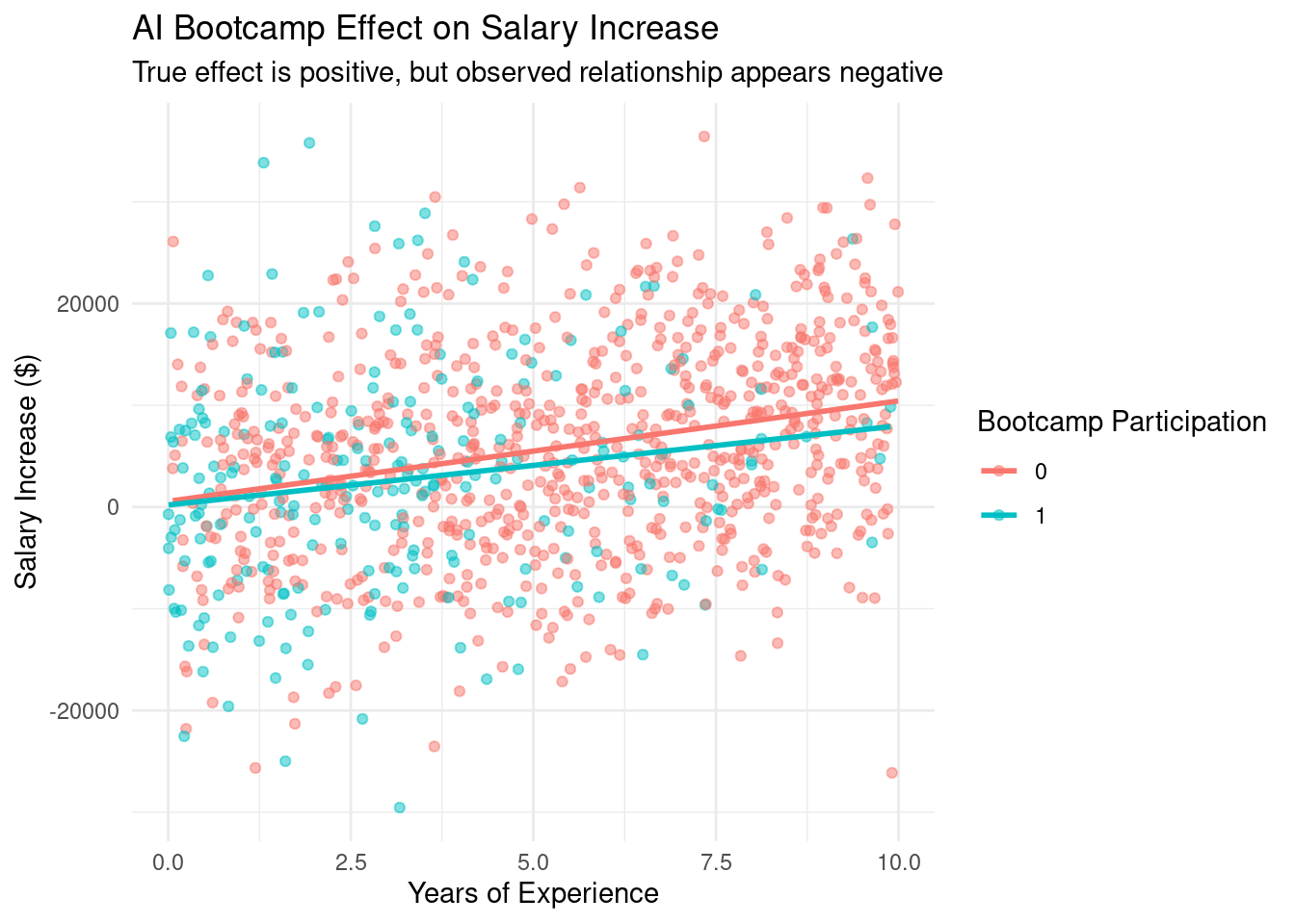
Cautionary tale: Unmeasured Confounders.

Imagine you’re a data scientist at the illustrious TechGiant Inc., a company that recently rolled out an intensive AI bootcamp program for its engineers. This ambitious initiative aims to elevate the workforce’s skills and propel innovation to new heights. You’ve been entrusted with a crucial task: to evaluate the program’s effectiveness by examining its impact on engineers’ salaries.

library(MatchIt)
library(dplyr)
library(ggplot2)
set.seed(123)

# Generate synthetic data
n <- 1000
experience <- runif(n, 0, 10)  # Years of experience
procrastination <- rnorm(n)  # Unobserved procrastination level
bootcamp <- rbinom(n, 1, plogis(-0.3 * experience + 0.5 * procrastination))  # Bootcamp participation
salary_increase <- 2000 * bootcamp + 1000 * experience - 9000 * procrastination + rnorm(n, 0, 5000)

# True average treatment effect is $2000

data <- data.frame(experience = experience,
                   bootcamp = bootcamp,
                   salary_increase = salary_increase)

# Naive estimate
naive_model <- lm(salary_increase ~ bootcamp, data = data)
naive_ate <- coef(naive_model)["bootcamp"]

# Matching on experience (ignoring unobserved procrastination)
m.out <- matchit(bootcamp ~ experience,
                 data = data,
                 method = "nearest",
                 ratio = 1)
matched_data <- match.data(m.out)

# Estimate ATT on the matched sample (1:1 matching pairs each treated participant)
matched_model <- lm(salary_increase ~ bootcamp,
                    data = matched_data,
                    weights = weights)
matched_att <- coef(matched_model)["bootcamp"]

# Print results
cat("True ATE / ATT: $2000\n")

True ATE / ATT: $2000

cat("Naive comparison estimate:", round(naive_ate, 2), "\n")

Naive comparison estimate: -3307.67 

cat("Matched estimate (ATT in matched sample):", round(matched_att, 2), "\n")

Matched estimate (ATT in matched sample): -1543.69 

# Visualize results
ggplot(data, aes(x = experience,
                 y = salary_increase,
                 color = factor(bootcamp))) +
  geom_point(alpha = 0.5) +
  geom_smooth(method = "lm", se = FALSE) +
  labs(title = "AI Bootcamp Effect on Salary Increase",
       subtitle = "True effect is positive, but observed relationship appears negative",
       x = "Years of Experience",
       y = "Salary Increase ($)",
       color = "Bootcamp Participation") +
  theme_minimal()

What’s happening in this scenario? Let’s break it down:

1. The True Impact: In reality, the bootcamp program is a success. It genuinely enhances skills and, consequently, leads to higher salary increases.
2. Experience and Participation: Less experienced engineers are more likely to enroll in the bootcamp, perhaps viewing it as a way to bridge the gap with their seasoned colleagues.
3. Procrastination as a Hidden Factor: These same less experienced engineers, possibly due to feeling overwhelmed or uncertain in their roles, tend to have higher levels of procrastination.
4. Motivation’s Influence on Salary: This inherent motivation leads to exceptional performance and subsequent salary raises, whether or not they participate in the bootcamp.
5. Matching Gone Awry: By focusing on matching solely based on experience and overlooking motivation, you inadvertently compare highly motivated non-participants with a mix of motivated and less motivated participants.

The consequence? Your analysis paints a deceptive picture, indicating a negative effect of the bootcamp when the true effect is, in fact, positive.

This example illustrates a critical lesson in causal inference: the danger of unmeasured confounders. In this case, motivation acts as an unmeasured confounder, influencing both the likelihood of bootcamp participation and salary increases. As a business data scientist, this scenario highlights the importance of:

1. Thinking critically about all factors that might influence both your treatment (bootcamp participation) and outcome (salary increases).
2. Recognizing the limitations of your data and analysis methods.
3. Communicating these nuances to stakeholders who might otherwise make decisions based on misleading results.
4. Considering additional data collection or alternative analysis methods to account for potential unmeasured confounders.

In the end, your role isn’t just to crunch numbers, but to uncover the true story behind the data and guide your company towards informed decisions. This might involve recommending a more comprehensive study that includes measures of motivation, or suggesting a randomized pilot program for future iterations of the bootcamp.

13.8 Conclusion: The Power and Pitfalls of Matching

Matching is a powerful tool in the causal inference toolkit, offering a way to construct valid comparison groups and tease out causal effects from observational data. However, as we’ve seen, it’s not without its complexities and potential pitfalls.

From the basic concept of pairing similar units to the intricacies of different distance measures and matching algorithms, we’ve explored the mechanics of how matching works. We’ve also delved into its limitations, illustrated vividly by the Ozzy Osbourne Conundrum, which reminds us that observable characteristics don’t always tell the full story.

The critique by King and Nielsen serves as a important cautionary tale, particularly regarding the use of propensity score matching. Their work underscores the importance of understanding the theoretical underpinnings of our methods and approaching them critically.

As data scientists, our task is to navigate these complexities, understanding when and how to apply matching methods appropriately. We must be aware of their strengths and limitations, always striving for transparency in our processes and robustness in our results.

Matching, when used judiciously, can be a powerful ally in our quest to uncover causal relationships. But like any tool, its effectiveness depends on the skill and understanding of those who wield it.

In later chapters on stochastic tree ensembles, we will see that propensity information plays an essential role even in flexible Bayesian modeling. As discussed in Bayesian Causal Forests, incorporating the estimated propensity score into the prognostic forest helps mitigate regularization-induced confounding (RIC) under the model’s assumptions. However, neither matching nor conditioning on a propensity score eliminates unmeasured confounding: if key covariates determining treatment assignment remain unobserved, observational estimates remain vulnerable to hidden bias.

TipLearn more

• Hernán and Robins (2016) Using Big Data to Emulate a Target Trial When a Randomized Trial Is Not Available.
• Ho et al. (2011) {MatchIt}: Nonparametric Preprocessing for Parametric Causal Inference.
• King and Nielsen (2019) Why Propensity Scores Should Not Be Used for Matching.

Hernán, Miguel A., and James M. Robins. 2016. “Using Big Data to Emulate a Target Trial When a Randomized Trial Is Not Available.” American Journal of Epidemiology 183 (8): 758–64. https://doi.org/10.1093/aje/kwv254.

Ho, Daniel E., Kosuke Imai, Gary King, and Elizabeth A. Stuart. 2011. “MatchIt: Nonparametric Preprocessing for Parametric Causal Inference.” Journal of Statistical Software 42 (8): 1–28. https://doi.org/10.18637/jss.v042.i08.

Ho, Daniel E, Kosuke Imai, Gary King, and Elizabeth A Stuart. 2007. “Matching as Nonparametric Preprocessing for Reducing Model Dependence in Parametric Causal Inference.” Political Analysis 15 (3): 199–236.

King, Gary, and Richard Nielsen. 2019. “Why Propensity Scores Should Not Be Used for Matching.” Political Analysis 27 (4): 435–54. https://doi.org/10.1017/pan.2019.11.