---
title: "Hurdle Models"
share:
permalink: "https://book.martinez.fyi/hurdle.html"
description: "Business Data Science: Hurdle Models"
linkedin: true
email: true
mastodon: true
---
<img src="img/hurdle.jpg" align="right" height="280" alt="Hurdle Models" />
## What are Hurdle Models and When are they Useful?
Hurdle models are a specialized statistical tool designed to handle data with a
preponderance of zero values, which often defy the assumptions of conventional
distributions like the normal or Poisson. These models are particularly valuable
when the data-generating process naturally consists of two distinct stages:
1. **Process 1: The Hurdle - Zero or Non-Zero?** This stage acts as the
gatekeeper, determining whether the underlying data-generating mechanism is
"active" or "dormant." It essentially answers the question: Is the outcome
zero or non-zero?
2. **Process 2: Modeling the Non-Zeros.** Contingent upon the outcome of
Process 1, if the result is non-zero, this second stage steps in to model
the specific value it assumes. The choice of distribution for this modeling
phase hinges on the nature of the data and could encompass lognormal, gamma,
Poisson, or negative binomial distributions.
Consider the scenario of analyzing user engagement with a new software feature.
Some users might never activate the feature, perhaps due to lack of awareness or
need. Others who find it valuable might use it to varying extents. A hurdle
model effectively captures both the probability of a user engaging with the
feature at all (Process 1 - crossing the 'hurdle'), and the extent of their
engagement if they do (Process 2 - the usage intensity).
### Mathematical Representation for a Hurdle Model with a Log Normal Component
Let's delve into the mathematical underpinnings, keeping it as intuitive as possible.
**Step 1: The Zero-Inflation Component**
* Let $Z_i$ be a binary indicator variable for whether observation $i$ is zero.
* $Z_i \sim Bernoulli(\theta_i)$
* where $\theta_i = logit^{-1}(\alpha_{zero} + \tilde{X}_i \beta_{zero} + \tau_{zero} T_i)$
* $\tilde{X}_i$ is the standardized design matrix (predictor variables) for observation $i$
* $T_i$ is the treatment indicator (1 for treatment, 0 for control).
* Priors:
* $\alpha_{zero} \sim Normal(\mu_{\alpha_{logit}}, \sigma_{\alpha_{logit}})$
* $\beta_{zero} \sim Normal(\mu_{\beta_{logit}}, \sigma_{\beta_{logit}})$
* $\tau_{zero} \sim Normal(\mu_{\tau_{logit}}, \sigma_{\tau_{logit}})$
**Log-Normal Component**
* Let $Y_i$ be the outcome variable.
* If $Z_i = 0$ (i.e., the outcome is zero), then $Y_i = 0$.
* If $Z_i = 1$ (i.e., the outcome is positive), then:
* $log(Y_i) \sim Normal(\mu_i, \sigma_{lnorm}^2)$
* where $\mu_i = \alpha_{lnorm} + \tilde{X}_i \beta_{lnorm} + \tau_{lnorm} T_i$
* Priors:
* $\alpha_{lnorm} \sim Normal(\mu_{log(y)}, 1)$
* $\beta_{lnorm} \sim Normal(0, 0.5)$
* $\tau_{lnorm} \sim Normal(\mu_{\tau}, \sigma_{\tau})$
* $\sigma_{lnorm} \sim Normal(0, 0.5)$
**Combined Model**
* The overall likelihood for observation $i$ is:
* $P(Y_i = 0) = \theta_i$
* $P(Y_i > 0) = (1 - \theta_i) \times \frac{1}{Y_i \sigma_{lnorm} \sqrt{2\pi}} exp \left( -\frac{(log(Y_i) - \mu_i)^2}{2 \sigma_{lnorm}^2} \right)$
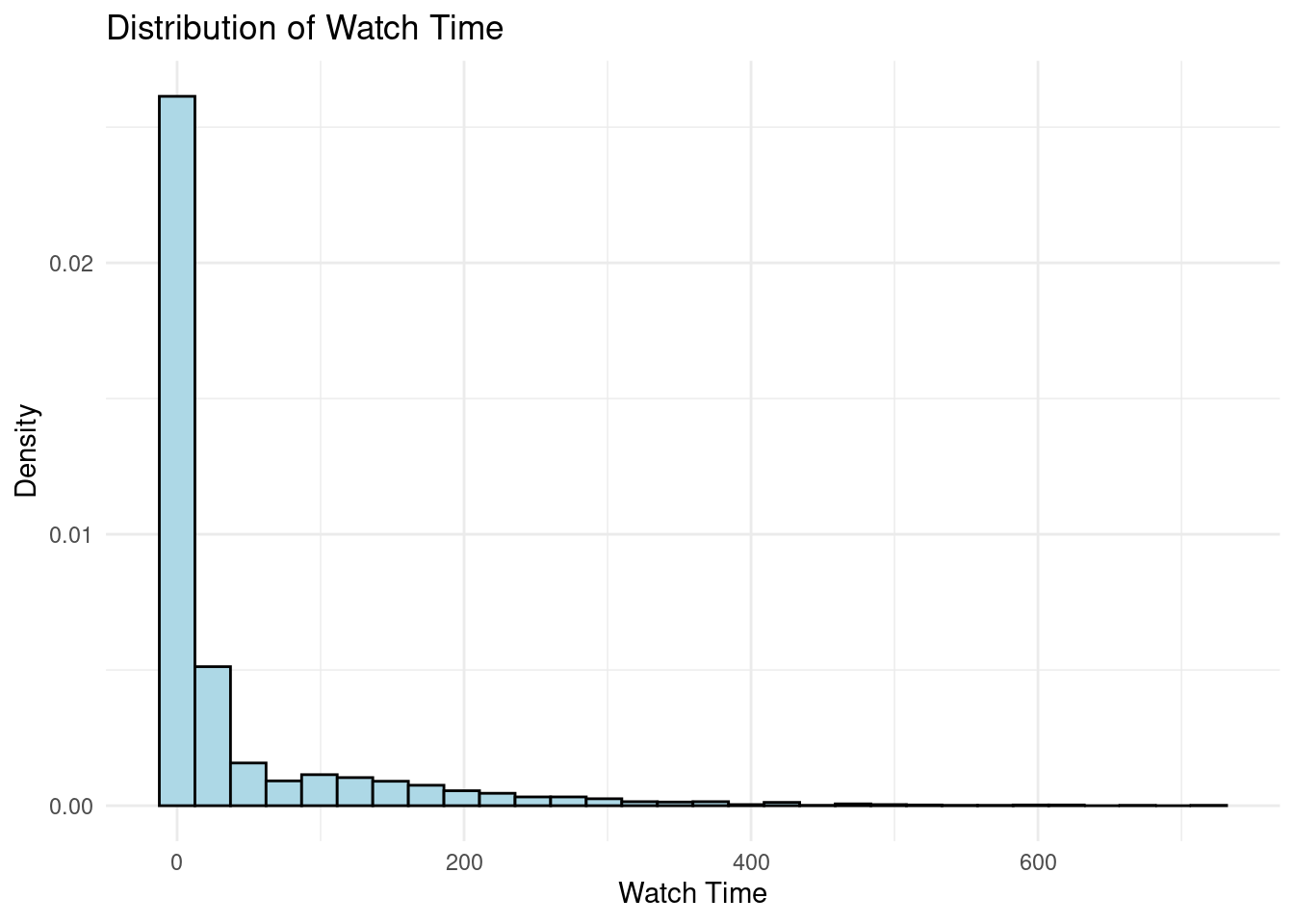
## Simulating Data for a Hurdle Model
Let's bring these concepts to life with a practical example. Imagine you're part
of an online video content company aiming to assess the impact of a novel
marketing strategy on video watch time. You notice that certain videos garner
substantial watch time, while others remain unwatched. To rigorously test this
new strategy, you randomly assign videos to either a treatment or control group.
Here's how we might simulate such data:
```{r message=FALSE, warning=FALSE}
library(dplyr)
set.seed(123)
n <- 3000

# Simulate covariates (unchanged)
fake_data <- data.frame(
  genre = sample(c("Comedy", "Education", "Music"), n, replace = TRUE),
  length = stats::rnorm(n, mean = 10, sd = 3),
  popular_channel = stats::rbinom(n, 1, 0.2)
)

# Treatment indicator (unchanged)
fake_data$treatment <- stats::rbinom(n, 1, 0.5)

# Model parameters (coefficients) - unchanged
beta_zero <- c(0.5, -0.2, 1)
beta_mean <- c(2, 0.1, 0.5)

# Modified treatment effect for zero probability
# We want P(zero | treated) = P(zero | control) - 0.05
# Assuming P(zero | control) = 0.3
p_zero_control <- 0.3
p_zero_treated <- p_zero_control - 0.05
treatment_effect_zero_prob <- qlogis(p_zero_treated) - qlogis(p_zero_control)

# Treatment effect for watch time
treatment_effect_watch_time <- 2

# Linear predictors (with modified treatment effect)
zero_prob_logit <- beta_zero[1] +
                   ifelse(fake_data$genre == "Education", beta_zero[2], 0) +
                   beta_zero[3] * fake_data$popular_channel +
                   treatment_effect_zero_prob * fake_data$treatment

log_normal_mean <- beta_mean[1] +
                   beta_mean[2] * fake_data$length +
                   beta_mean[3] * fake_data$popular_channel +
                   treatment_effect_watch_time * fake_data$treatment

# Generate potential outcomes
fake_data <- within(fake_data, {
    zero_prob_control <- stats::plogis(zero_prob_logit - treatment_effect_zero_prob * treatment)
    zero_prob_treated <- stats::plogis(zero_prob_logit)
    watch_time_control <- ifelse(stats::rbinom(n, 1, 1 - zero_prob_control) == 1,
                                 stats::rlnorm(n, log_normal_mean - treatment_effect_watch_time * treatment, 0.5),
                                 0)
    watch_time_treated <- ifelse(stats::rbinom(n, 1, 1 - zero_prob_treated) == 1,
                                 stats::rlnorm(n, log_normal_mean, 0.5),
                                 0)
    # Calculate treatment effects
    tau_watch_time <- watch_time_treated - watch_time_control
    tau_zero_prob <- zero_prob_treated - zero_prob_control
    # Observed outcome based on treatment assignment
    zero_prob <- ifelse(treatment == 1, zero_prob_treated, zero_prob_control)
    watch_time <- ifelse(treatment == 1, watch_time_treated, watch_time_control)
}) |>
  dplyr::mutate(treatment = as.logical(treatment))


dplyr::glimpse(fake_data)
```
```{r}
library(ggplot2)
ggplot(fake_data, aes(x = watch_time)) +
  geom_histogram(aes(y = after_stat(density)), bins = 30, fill = "lightblue", color = "black") +
  labs(title = "Distribution of Watch Time", x = "Watch Time", y = "Density") +
  theme_minimal()
```
In this simulated data, the average treatment effect leads to an increase in
watch time of approximately `r round(mean(fake_data$tau_watch_time))` hours.
Additionally, the probability of having zero hours of watch time decreases by
`r round(100*mean(fake_data$tau_zero_prob))` percentage points.
## Pitfalls of Naive OLS Regression
Since treatment assignment is random in our simulation, it might be
tempting to use a simple linear regression:
```{r}
lm1 <- lm(data = fake_data,
   watch_time ~ genre + popular_channel + length + treatment) |>
  broom::tidy(conf.int = TRUE)

lm1
```
However, this approach overestimates the true treatment effect. The
point estimate and confidence intervals are significantly higher than
the actual impact.
Another common approach is to log-transform the outcome variable and
then apply OLS:
```{r}
# Run the OLS regression with log(watch_time + 1) as the dependent variable
lm2 <- lm(data = fake_data, log(watch_time + 1) ~ genre +
            popular_channel + length + treatment) |>
  broom::tidy(conf.int = TRUE)

lm2
mean_watch_time_control <- mean(fake_data$watch_time[fake_data$treatment == FALSE])

point_estimate <- mean_watch_time_control*(1+lm2$estimate[6])
lb <- mean_watch_time_control*(1+lm2$conf.low[6])
ub <- mean_watch_time_control*(1+lm2$conf.high[6])
```
In this case, the point estimate (`r round(point_estimate)`) and the
confidence interval ([`r round(lb)`, `r round(ub)`]) underestimate the
true effect.
## Bayesian Hurdle Model Using {imt}
<img src="https://raw.githubusercontent.com/google/imt/refs/heads/main/man/figures/logo.png" align="right" height="138" alt="logo of the imt package" />
Let's use the [{imt}](https://github.com/google/imt) package to fit a Bayesian
hurdle model:
```{r fit, message=FALSE, results = "hide"}
library(imt)

# Create the hurdleLogNormal object
model <- hurdleLogNormal$new(
  data = fake_data,
  y = "watch_time",
  x = c("length", "popular_channel", "genre"),
  treatment = "treatment",
  tau_mean_logit = 0,
  tau_sd_logit = 0.5,
  mean_tau = 0,
  sigma_tau = 0.035
)
```
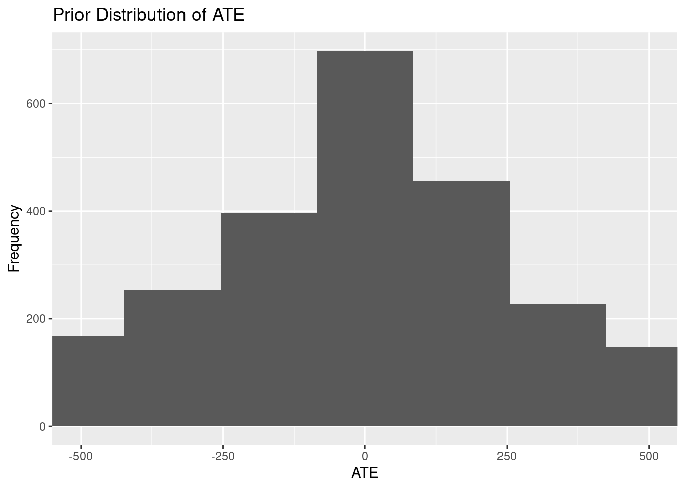
### Plot Priors
Before diving into the posterior analysis, let's visualize the priors we've set
for our model:
```{r}
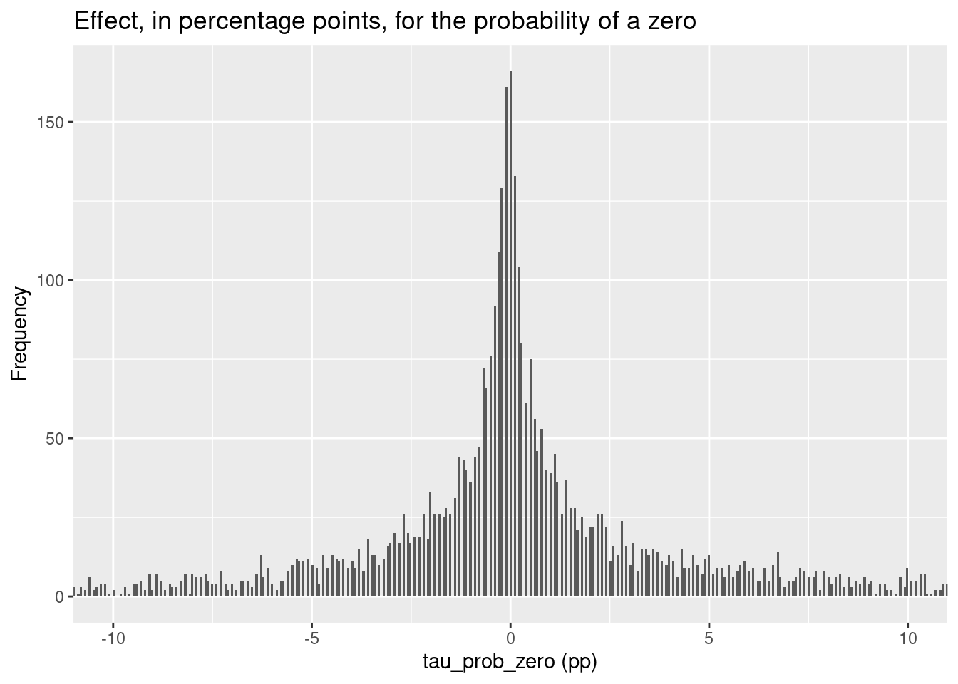
prior_plots <- model$plotPrior(bins = 1000,
                               xlim_ate = c(-500, 500),
                               xlim_tau = c(-10, 10))

# To display the plots:
prior_plots$ate_prior
prior_plots$tau_prior
```
These plots provide a visual representation of our prior beliefs about the
treatment effects before observing the data.
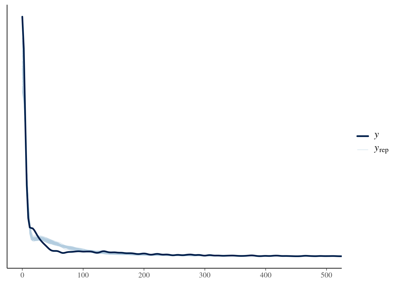
### Posterior Analysis
Now, let's examine the posterior distribution and assess the model's fit:
```{r}
ppc_plot <- model$posteriorPredictiveCheck(n = 50, xlim = c(0, 500))
ppc_plot # Display the plot
```
The posterior predictive check helps us gauge whether the model adequately
captures the characteristics of the observed data.
Finally, let's extract the key estimates:
```{r}
# Get ATE point estimate and credible interval
ate <- model$pointEstimate("ATE")
ci_statement <- model$credibleInterval("ATE")

# Print results
cat("The mean of the posterior distribution of the average treatment effect is",
    round(ate))
ci_statement
```
```{r}
# Get ATE point estimate and credible interval
tau_prob_zero <- model$pointEstimate("tau_prob_zero")
ci_statement <- model$credibleInterval("tau_prob_zero")

# Print results
cat("The mean of the posterior distribution of the effect on the probability of a zero is",
    round(tau_prob_zero,4))
ci_statement
```
```{r}
model$calcProb(effect_type = "ATE", a = 29)
```
The Bayesian hurdle model, as implemented with {imt}, provides a more nuanced
and accurate assessment of the treatment effect in the presence of excessive
zeros, outperforming naive OLS approaches.
## Hurdle vs. Zero-Inflated Models: Choosing the Right Tool for the Job
While hurdle models excel at handling data with excess zeros, it's crucial to
distinguish them from another class of models designed for similar scenarios:
zero-inflated models. Both tackle the challenge of zero inflation, but they do
so with subtle yet important differences.
### Conceptual Differences
- **Hurdle Models:** Assume a single process generates both zeros and
non-zeros. The "hurdle" represents a threshold that must be crossed before
any non-zero outcome can occur. Think of it as a binary decision: either the
outcome is zero, or it's something positive that we then model with a
suitable distribution.
- **Zero-Inflated Models:** Assume two distinct processes are at play. One
process generates only zeros (the "structural zeros"), while another process
generates both zeros and non-zeros (the "count process"). This allows for
the possibility of "excess zeros" beyond what would be expected from the
count process alone.
### When to Use Each
- **Hurdle Models:** Ideal when there's a clear conceptual hurdle or threshold
that needs to be overcome before a non-zero outcome can happen. For
instance, in our video watch time example, users need to decide to watch a
video at all before any watch time can be recorded.
- **Zero-Inflated Models:** More suitable when you suspect there are two
fundamentally different types of zeros in your data. For example, in a
survey about alcohol consumption, some respondents might be teetotalers
(structural zeros), while others might simply not have consumed alcohol
during the survey period (zeros from the count process).
The choice between a hurdle model and a zero-inflated model hinges on your
understanding of the data-generating process and the research question at hand.
If you believe there's a single process with a clear hurdle, a hurdle model is
the way to go. If you suspect multiple processes leading to zeros, a
zero-inflated model might be more appropriate.
In our video watch time example, we opted for a hurdle model because the
decision to watch a video (or not) seemed like a natural hurdle. However, if we
had reason to believe that some videos were inherently unappealing and would
never be watched by anyone (structural zeros), a zero-inflated model might have
been worth considering.
The key takeaway is that both hurdle and zero-inflated models offer powerful
ways to handle excess zeros, but their underlying assumptions and
interpretations differ.
By carefully considering the nature of your data and your research goals, you
can choose the model that best suits your needs and unlocks valuable insights
hidden within the zeros.
::: {.callout-tip}
## Learn more
- @mc-stan2024finite Stan User's Guide: Finite Mixtures and Zero-inflated Models.
- @heiss2022hurdle: A guide to modeling outcomes that have lots of zeros with Bayesian hurdle lognormal and hurdle Gaussian regression models.
:::