14 Bayesian Synthetic Control

Synthetic control methods have become a widely applied tool for empirical researchers to estimate the effect of interventions or treatments, especially when traditional randomized controlled trials aren’t feasible. In a recent Journal of Economic Perspectives survey on the econometrics of policy evaluation, Susan Athey and Guido Imbens describe synthetic controls as “arguably the most important innovation in the policy evaluation literature in the last 15 years” (Athey and Imbens 2017). The technique involves creating a “synthetic” version of the treated unit by weighting untreated units from a donor pool. This essentially allows us to estimate what would have happened if the treatment had never occurred.

14.1 Key Concepts and Principles

Before we dive into the Bayesian approach, let’s review some fundamental concepts:

Pre-treatment Fit: The credibility of a synthetic control estimator hinges on how well it can track the trajectory of the outcome variable for the treated unit before the intervention. A close pre-treatment fit makes for more reliable post-treatment estimates.

Convex Hull Condition: The synthetic control method works best when the characteristics of the treated unit fall within the convex hull of the donor pool units’ characteristics. This ensures that the treated unit can be approximated by a weighted average of donor units.

Sparse Solutions: Synthetic control estimates typically involve only a few donor pool units with non-zero weights. This sparsity aids in interpretability and helps reduce overfitting.

No Anticipation: The method assumes that there are no anticipation effects before the intervention. If such effects exist, it’s advisable to backdate the intervention in the dataset.

Sufficient Pre- and Post-intervention Information: The credibility of the estimates depends on having enough pre-intervention periods to establish a good fit and enough post-intervention periods to observe the full effect of the intervention.

No Interference: The method assumes that the intervention does not affect the outcomes of the untreated units. This assumption should be carefully considered in the study design.

14.2 The Bayesian Advantage

Prior Information: Bayesian methods allow us to incorporate prior knowledge or beliefs about the data. This can be particularly useful when we have relevant information from past studies or expert opinions.

Posterior Distribution: By combining the prior distribution with the likelihood of the observed data, we get a posterior distribution. This distribution represents our updated beliefs about the parameters after taking into account the new data.

Uncertainty Quantification: One of the key strengths of Bayesian methods is their ability to quantify uncertainty. The posterior distribution gives us a range of plausible values for the treatment effects, along with associated probabilities.

Hierarchical Models: Bayesian synthetic control models can be built with hierarchical structures. This allows for more complex relationships and dependencies within the data.

Mathematical Formulation

In the Bayesian approach, we typically use a Dirichlet distribution as the prior for the weights, ensuring they are positive and sum to 1. We can also introduce a scaling matrix, often denoted as Γ, to control the importance of different predictors.

Let’s formalize this with some notation:

$X_1$: A $k \times 1$ matrix of predictors for the treated unit.
$X_0$: A $k \times J$ matrix of predictors for the donor units.
$w$: A $J\times 1$ vector of weights for the synthetic control.
$\sigma$: A scaling parameter.
$\Gamma$ A $k \times k$ scaling matrix.

A simple Bayesian synthetic control model can be formulated as:

\[ \begin{aligned} X_1 | w, \sigma &\sim N(X_0w , \text{diag}(\Gamma)^{-2}\sigma^2) \\ w &\sim \text{Dir}(1)\\ \sigma &\sim N^+(0,1)\\ \Gamma &\sim Dir((v_1, \dots, v_k)') \quad \text{s.t. } 1'v = 1 \\ \end{aligned} \]

Practical Implementation: The German Re-unification Example

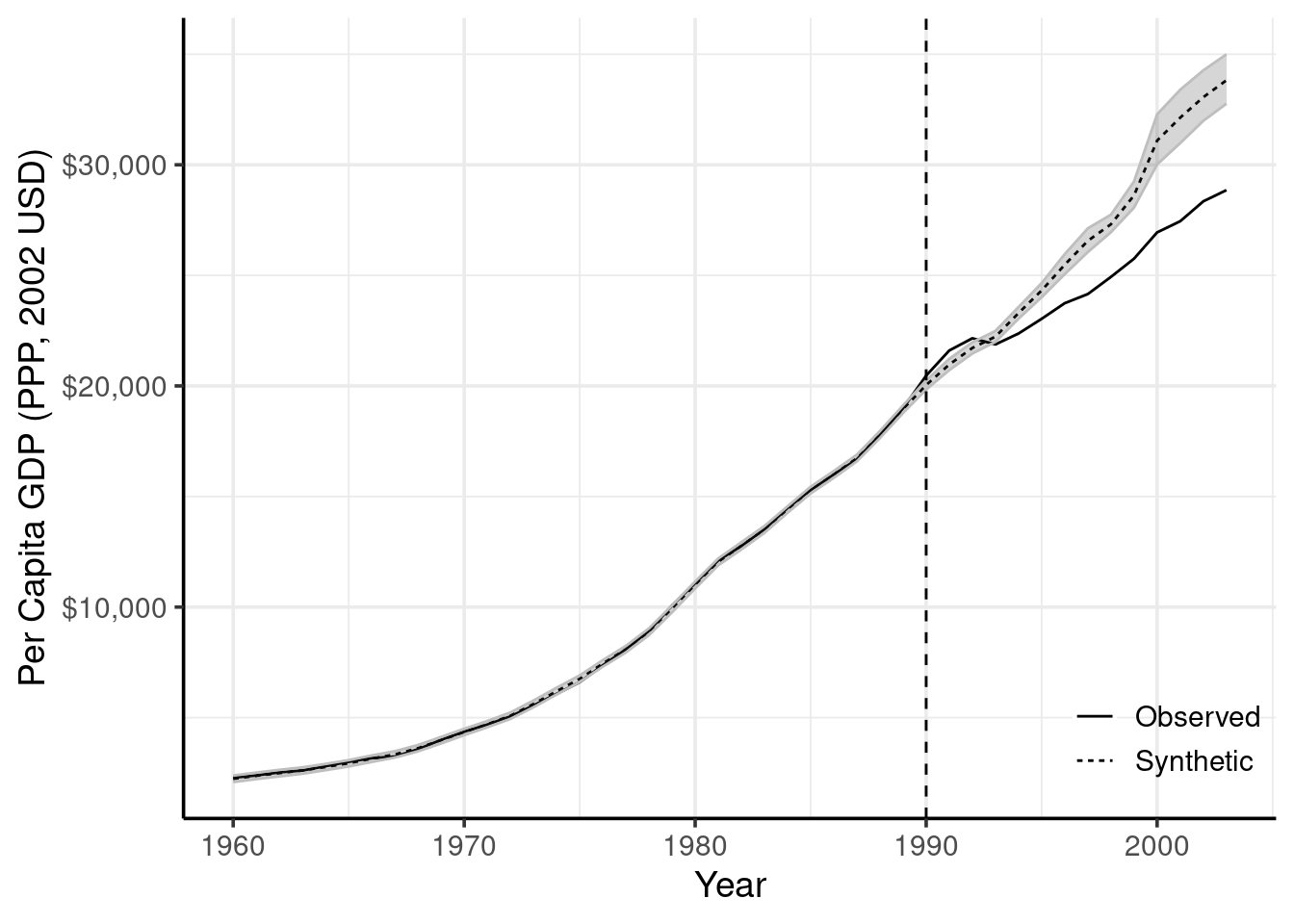
In 1989, a monumental event occurred: the reunification of East and West Germany. A natural question for policymakers was: “What impact did reunification have on West Germany’s GDP?”

This very question was addressed in one of the seminal papers on synthetic control (see Abadie, Diamond, and Hainmueller 2015). Using a Bayesian approach, we can not only estimate the effect of reunification but also quantify the uncertainty around that estimate.

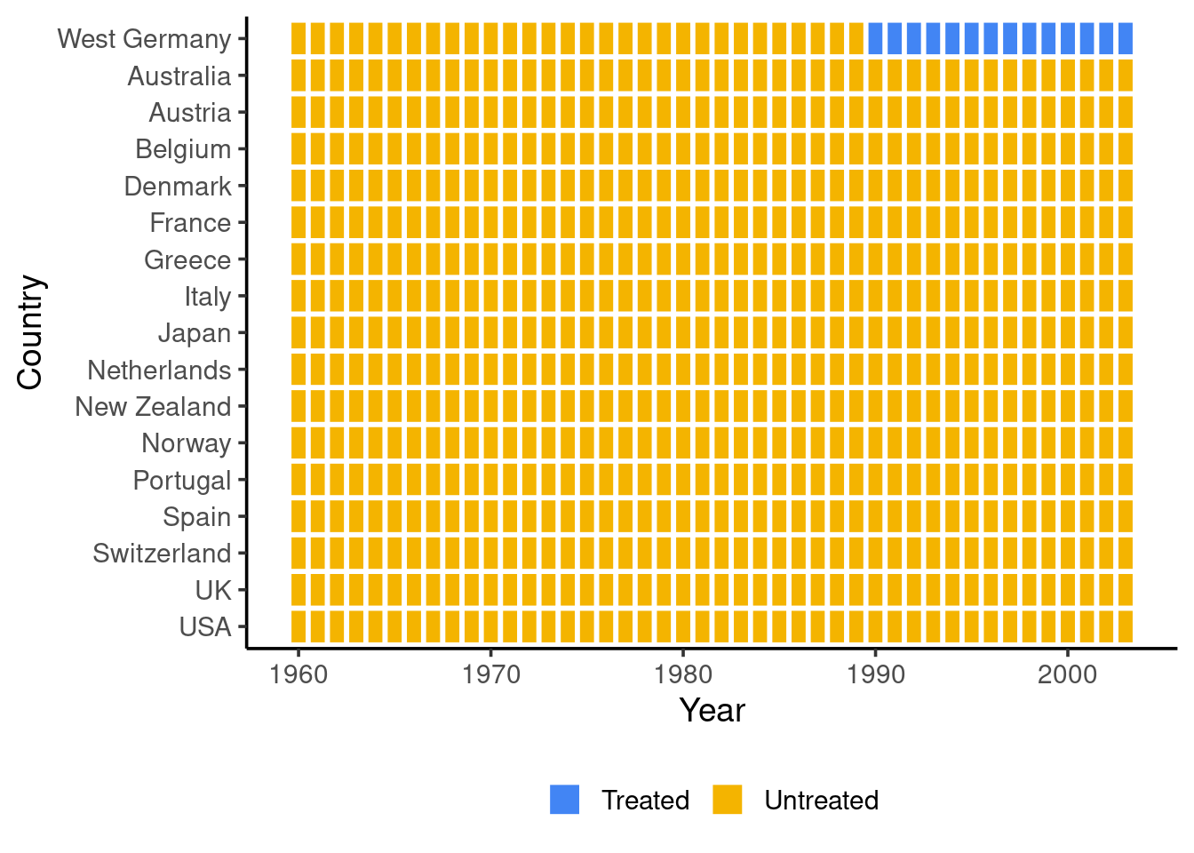
The {bsynth} package in R provides a convenient way to apply Bayesian synthetic control methods. Let’s see how we can analyze the German reunification data:

library("bsynth")
load("germany.rda")
germany_synth <- bayesianSynth$new(data = germany,
                                   time = year,
                                   id = country,
                                   treated = D,
                                   outcome = gdp,
                                   ci_width = 0.95,
                                   predictor_match = FALSE)

Transforming data

germany_synth$timeTiles + ggplot2::xlab("Year") + ggplot2::ylab("Country")

In this example, we’re starting with a simple model that doesn’t include predictor matching. We’ll fit the model and visualize the results:

germany_synth$fit(cores = 4)

# Vizualize the Bayesian Synthetic Control
germany_synth$synthetic + 
  ggplot2::xlab("Year") +
  ggplot2::ylab("Per Capita GDP (PPP, 2002 USD)") +
  ggplot2::scale_y_continuous(labels=scales::dollar_format())

We can also examine the estimated lift (the cumulative effect of the treatment) over a specific time period:

germany_synth$liftDraws(from = lubridate::as_date("1990-01-01"), 
                        to = lubridate::as_date("2002-01-01"))

When Things Go Wrong: The Pitfalls of Synthetic Controls

It’s crucial to remember that synthetic control isn’t a magic bullet. Things can go awry, and you could end up with estimates that are entirely off the mark. Here are some common pitfalls to watch out for:

Poor Pre-treatment Fit: If your synthetic control doesn’t accurately replicate the treated unit’s pre-treatment behavior, don’t use it. It’s as simple as that.
Overfitting: Even with a perfect pre-treatment fit, there’s the danger of overfitting. This is more likely to happen if you have a short pre-treatment period, a large donor pool, noisy data, or if you relax the weight constraints and allow for extrapolation.

Be careful when using synthetic controls, things co go bad and you could end up with an estimate that is the wrong sign!! The weight restriction allows us to cleanly characterize an upper bound for the bias:

\[\begin{align*} E[|\hat{\tau}_{1t} - \tau_{1t}|] \lesssim \underbrace{C_1\mathbb{E}\text{MAD}\left(Y_1^P, \hat{Y}_j^P\right) + k C_2 \mathbb{E}\text{MAD}\left(Z_1^1,\hat{Z}_j^1\right)}_{\text{First Order}} + \underbrace{C_3 J^{1/3} \frac{\bar{\sigma}}{T_0^{1/2}}}_{\text{Second Order}} \end{align*}\]

Fit matters most: If the synthetic control can not replicate the treated unit over time, you should not use it.
Don’t chase noise: Even with perfect pre-treatment fit there is the danger that you are over-fitting to the pre-treatment period.

Over-fitting is more likely in the following situations:

You have a short pre-treatment period (small $T_0$).
You have a large donor pool (large $J$) or the units are not similar to your treated unit.
You have very noisy data.
You allow for extrapolation by relaxing the weight constraints. In this case, you might have perfect pre-treatment fit but you will likely have significant bias from over-fitting.

Check the Bias of your Bayesian Synthetic Controls

The ‘bsynth’ package offers you a nice and easy way to check how likely it is that your estimate is badly biased! By computing an upper bound on the relative bias we get an estimate of the probability that your effect could change signs because of the bias.

In the case of the German re-unification this is unlikely when we consider the full post-treatment period of 12 years.

germany_synth$biasDraws(small_bias = 0.2, 
                        firstT = lubridate::as_date("1990-01-01"), 
                        lastT = lubridate::as_date("2002-01-01"))

However, for a smaller time frame of just 5 years after the re-unification, the bias could overturn the effect! Be careful when you choose a time period to measure cumulative effects as it will change the relative bias too.

germany_synth$biasDraws(small_bias = 0.2, 
                        firstT = lubridate::as_date("1990-01-01"), 
                        lastT = lubridate::as_date("1994-01-01"))

Learn more

Abadie (2021) Using Synthetic Controls: Feasibility, Data Requirements, and Methodological Aspects.
Abadie and Vives-i-Bastida (2022) Synthetic Controls in Action.
Martinez and Vives-i-Bastida (2023) Bayesian and Frequentist Inference for Synthetic Controls.

--- title: "Bayesian Synthetic Control" share: permalink: "https://book.martinez.fyi/bsynth.html" description: "Business Data Science: What Does it Mean to Be Data-Driven?" linkedin: true email: true mastodon: true --- Synthetic control methods have become a widely applied tool for empirical researchers to estimate the effect of interventions or treatments, especially when traditional randomized controlled trials aren't feasible. In a recent Journal of Economic Perspectives survey on the econometrics of policy evaluation, Susan Athey and Guido Imbens describe synthetic controls as "arguably the most important innovation in the policy evaluation literature in the last 15 years" [@athey2017state]. The technique involves creating a "synthetic" version of the treated unit by weighting untreated units from a donor pool. This essentially allows us to estimate what would have happened if the treatment had never occurred. ## Key Concepts and Principles Before we dive into the Bayesian approach, let's review some fundamental concepts: **Pre-treatment Fit:** The credibility of a synthetic control estimator hinges on how well it can track the trajectory of the outcome variable for the treated unit before the intervention. A close pre-treatment fit makes for more reliable post-treatment estimates. **Convex Hull Condition:** The synthetic control method works best when the characteristics of the treated unit fall within the convex hull of the donor pool units' characteristics. This ensures that the treated unit can be approximated by a weighted average of donor units. **Sparse Solutions:** Synthetic control estimates typically involve only a few donor pool units with non-zero weights. This sparsity aids in interpretability and helps reduce overfitting. **No Anticipation:** The method assumes that there are no anticipation effects before the intervention. If such effects exist, it's advisable to backdate the intervention in the dataset. **Sufficient Pre- and Post-intervention Information:** The credibility of the estimates depends on having enough pre-intervention periods to establish a good fit and enough post-intervention periods to observe the full effect of the intervention. **No Interference:** The method assumes that the intervention does not affect the outcomes of the untreated units. This assumption should be carefully considered in the study design. ## The Bayesian Advantage **Prior Information:** Bayesian methods allow us to incorporate prior knowledge or beliefs about the data. This can be particularly useful when we have relevant information from past studies or expert opinions. **Posterior Distribution:** By combining the prior distribution with the likelihood of the observed data, we get a posterior distribution. This distribution represents our updated beliefs about the parameters after taking into account the new data. **Uncertainty Quantification:** One of the key strengths of Bayesian methods is their ability to quantify uncertainty. The posterior distribution gives us a range of plausible values for the treatment effects, along with associated probabilities. **Hierarchical Models:** Bayesian synthetic control models can be built with hierarchical structures. This allows for more complex relationships and dependencies within the data. ### Mathematical Formulation In the Bayesian approach, we typically use a Dirichlet distribution as the prior for the weights, ensuring they are positive and sum to 1. We can also introduce a scaling matrix, often denoted as Γ, to control the importance of different predictors. Let's formalize this with some notation: - $X_1$: A $k \times 1$ matrix of predictors for the treated unit. - $X_0$: A $k \times J$ matrix of predictors for the donor units. - $w$: A $J\times 1$ vector of weights for the synthetic control. - $\sigma$: A scaling parameter. - $\Gamma$ A $k \times k$ scaling matrix. A simple Bayesian synthetic control model can be formulated as: $$ \begin{aligned} X_1 | w, \sigma &\sim N(X_0w , \text{diag}(\Gamma)^{-2}\sigma^2) \\ w &\sim \text{Dir}(1)\\ \sigma &\sim N^+(0,1)\\ \Gamma &\sim Dir((v_1, \dots, v_k)') \quad \text{s.t. } 1'v = 1 \\ \end{aligned} $$ ### Practical Implementation: The German Re-unification Example In 1989, a monumental event occurred: the reunification of East and West Germany. A natural question for policymakers was: "What impact did reunification have on West Germany's GDP?" This very question was addressed in one of the seminal papers on synthetic control [see @abadie2015comparative]. Using a Bayesian approach, we can not only estimate the effect of reunification but also quantify the uncertainty around that estimate. The {bsynth} package in R provides a convenient way to apply Bayesian synthetic control methods. Let's see how we can analyze the German reunification data: ```{r germany} library("bsynth") load("germany.rda") germany_synth <- bayesianSynth$new(data = germany, time = year, id = country, treated = D, outcome = gdp, ci_width = 0.95, predictor_match = FALSE) germany_synth$timeTiles + ggplot2::xlab("Year") + ggplot2::ylab("Country") ``` In this example, we're starting with a simple model that doesn't include predictor matching. We'll fit the model and visualize the results: ```{r fit, message=FALSE, results = "hide"} germany_synth$fit(cores = 4) # Vizualize the Bayesian Synthetic Control germany_synth$synthetic + ggplot2::xlab("Year") + ggplot2::ylab("Per Capita GDP (PPP, 2002 USD)") + ggplot2::scale_y_continuous(labels=scales::dollar_format()) ``` ::: {.content-visible when-format="html"} We can also examine the estimated lift (the cumulative effect of the treatment) over a specific time period: ```{r liftDraws} #| eval: !expr knitr::is_html_output() germany_synth$liftDraws(from = lubridate::as_date("1990-01-01"), to = lubridate::as_date("2002-01-01")) ``` ::: ### When Things Go Wrong: The Pitfalls of Synthetic Controls It's crucial to remember that synthetic control isn't a magic bullet. Things can go awry, and you could end up with estimates that are entirely off the mark. Here are some common pitfalls to watch out for: - **Poor Pre-treatment Fit:** If your synthetic control doesn't accurately replicate the treated unit's pre-treatment behavior, don't use it. It's as simple as that. - **Overfitting:** Even with a perfect pre-treatment fit, there's the danger of overfitting. This is more likely to happen if you have a short pre-treatment period, a large donor pool, noisy data, or if you relax the weight constraints and allow for extrapolation. **Be careful** when using synthetic controls, things co go bad and you could end up with an estimate that is the wrong sign!! The weight restriction allows us to cleanly characterize an upper bound for the bias: \begin{align*} E[|\hat{\tau}_{1t} - \tau_{1t}|] \lesssim \underbrace{C_1\mathbb{E}\text{MAD}\left(Y_1^P, \hat{Y}_j^P\right) + k C_2 \mathbb{E}\text{MAD}\left(Z_1^1,\hat{Z}_j^1\right)}_{\text{First Order}} + \underbrace{C_3 J^{1/3} \frac{\bar{\sigma}}{T_0^{1/2}}}_{\text{Second Order}} \end{align*} 1. **Fit matters most**: If the synthetic control can not replicate the treated unit over time, you should **not** use it. 2. **Don't chase noise**: Even with perfect pre-treatment fit there is the danger that you are **over-fitting** to the pre-treatment period. Over-fitting is more likely in the following situations: - You have a short pre-treatment period (small $T_0$). - You have a large donor pool (large $J$) or the units are not similar to your treated unit. - You have very noisy data. - You allow for extrapolation by relaxing the weight constraints. In this case, you might have perfect pre-treatment fit but you will likely have significant bias from over-fitting. ### Check the Bias of your Bayesian Synthetic Controls The 'bsynth' package offers you a nice and easy way to check how likely it is that your estimate is badly biased! By computing an upper bound on the relative bias we get an estimate of the probability that your effect could change signs because of the bias. In the case of the German re-unification this is unlikely when we consider the full post-treatment period of 12 years. ::: {.content-visible when-format="html"} ```{r bias1, warning=FALSE} #| eval: !expr knitr::is_html_output() germany_synth$biasDraws(small_bias = 0.2, firstT = lubridate::as_date("1990-01-01"), lastT = lubridate::as_date("2002-01-01")) ``` ::: However, for a smaller time frame of just 5 years after the re-unification, the bias could overturn the effect! Be careful when you choose a time period to measure cumulative effects as it will change the relative bias too. ::: {.content-visible when-format="html"} ```{r bias2, warning=FALSE} #| eval: !expr knitr::is_html_output() germany_synth$biasDraws(small_bias = 0.2, firstT = lubridate::as_date("1990-01-01"), lastT = lubridate::as_date("1994-01-01")) ``` ::: ::: {.callout-tip} ## Learn more - @abadie2021using Using Synthetic Controls: Feasibility, Data Requirements, and Methodological Aspects. - @abadie2022synthetic Synthetic Controls in Action. - @martinez2023bayesian Bayesian and Frequentist Inference for Synthetic Controls. :::