---
title: "LongBet: From Effects to Decisions"
description: "Turning dynamic treatment effects into decisions: annual dollar valuations per seller, a ranked rollout under a capacity constraint, targeting when effects vary across units, and a joint screen over three outcomes at once."
format:
html:
css: longbet.css
share:
permalink: "https://book.martinez.fyi/longbet_decisions.html"
description: "LongBet: from dynamic effects to business decisions"
linkedin: true
email: true
mastodon: true
---
::: {.callout-note title="Continues the marketplace rollout"}
This chapter continues the randomized rollout of **[LongBet: Dynamic Treatment Effects in Staggered Rollouts](longbet.qmd)**, reusing its sellers, calendar and fitted model. The comparison with the econometric estimators follows in **[LongBet and Modern Difference-in-Differences](longbet_did.qmd)**, and forecasting in **[LongBet: Forecasting and Observational Panels](longbet_extensions.qmd)**.
:::
```{r setup}
#| message: false
#| warning: false
library(longbet)
library(dplyr)
library(tidyr)
library(tibble)
library(ggplot2)
library(purrr)
library(knitr)

source("R/longbet-common.R")
source("R/longbet-sim.R")
source("R/longbet-artifacts.R")
verify_longbet_environment()
theme_set(theme_minimal(base_size = 12))

ro <- simulate_rollout()
list2env(ro[c("n", "week_study", "weeks_all", "listings", "level_i", "a_i", "mu0_true",
              "tau_true", "x", "sd_eps", "z_train", "broad")], environment())
lb_fit <- lb_core_fit(ro)
```
## The Decision {#sec-longbet-decision}
The marketplace keeps 12% of GMV and the optimizer costs \$500 per seller per year. An effect estimate becomes a dollar figure only after three choices, and each one should be visible in the code rather than buried in a spreadsheet:
1. **A baseline revenue path.** Here it is the model's fitted untreated outcome over the last four study weeks, including the seller's own intercept, converted from logs and held flat for the year.
2. **A trajectory over the decision horizon.** The model's own twelve-week path, then the week-12 effect held for the remaining forty weeks.
3. **A decision rule.** Rank by posterior median net value, or require a probability of profitability, or treat everyone.
The first two are assumptions. The third is the actual decision. Keeping them separate is what lets the sensitivity table later change one at a time.
```{r common-launch}
#| message: false
z_all <- matrix(as.integer(week_study >= 9), n, length(week_study), byrow = TRUE)
S_target <- sum(week_study >= 9)
pred_all <- predict(lb_fit, x = x, z = z_all, t = week_study, random_seed = 1)
tau_hat_draws <- pred_all$tauhats[, ncol(z_all), ]
recent <- tail(seq_along(week_study), 4)
sigma2_hat <- median(as.numeric(lb_fit$sigma0_draws))^2 * lb_fit$sdy^2
mu0_hat <- apply(pred_all$muhats0[, recent, , drop = FALSE], c(1, 2), median)
gmv_week <- rowMeans(exp(mu0_hat + sigma2_hat / 2))
initial_lift <- apply(expm1(pred_all$tauhats[, which(week_study >= 9), , drop = FALSE]), c(1, 3), sum)
```
A log effect becomes a proportional lift through $e^{\tau} - 1$, and the conversion happens **inside every draw** before anything is averaged, because $e^{\bar\tau} - 1$ is not the average of $e^{\tau} - 1$. That is the single most common way a log-scale model gets misreported to a business audience.
```{r economics}
TAKE_RATE <- 0.12; ANNUAL_COST <- 500; HOLD_WEEKS <- 52 - S_target
annual_lift <- initial_lift + HOLD_WEEKS * expm1(tau_hat_draws)   # weeks of baseline revenue gained
net_draws   <- TAKE_RATE * gmv_week * annual_lift - ANNUAL_COST   # dollars per seller per year
median_net <- apply(net_draws, 1, median); p_worth <- rowMeans(net_draws > 0)

# The simulator's own baseline and effects, used only to score the policies afterwards.
gmv_week_true <- rowMeans(exp(mu0_true[, week_study[recent]] + sd_eps^2 / 2))
true_annual_lift <- rowSums(expm1(outer(a_i, seq_len(S_target), function(a, s) a * h_shape(s)))) +
  HOLD_WEEKS * expm1(a_i * h_shape(S_target))
net_true <- TAKE_RATE * gmv_week_true * true_annual_lift - ANNUAL_COST
tibble(Quantity = c("Median estimated weekly baseline GMV", "Median simulator baseline (scoring only)",
                    "Median break-even annual lift"),
       Value = c(scales::dollar(median(gmv_week)), scales::dollar(median(gmv_week_true)),
                 scales::percent(median(ANNUAL_COST / (TAKE_RATE * 52 * gmv_week)), 0.1))) %>%
  kable(caption = "The baseline estimate and the break-even lift it implies for the median seller.")
```
Notice what the break-even lift does to the problem. The cost is flat per seller and the benefit scales with the seller's revenue, so a large seller clears the bar with a much smaller percentage lift than a small one. The targeting question is therefore never "who responds most", it is "who is worth it".
## Ranking Sellers Under a Capacity Constraint
The onboarding team can migrate about 80 sellers a week. A ranked list is the deliverable, and the posterior gives several defensible ways to build one.
```{r policy-table}
by_value <- order(median_net, decreasing = TRUE)
top_k <- function(K) {
  keep <- rep(FALSE, n); eligible <- by_value[median_net[by_value] > 0]
  keep[head(eligible, min(K, length(eligible)))] <- TRUE; keep
}
policies <- list(
  "Do not roll out" = rep(FALSE, n),
  "Roll out to everyone" = rep(TRUE, n),
  "Broad catalogs (>= 50 listings)" = broad,
  "Up to 80 sellers by median net value" = top_k(80),
  "Up to 160 sellers by median net value" = top_k(160),
  "Positive median net value (uncapped)" = median_net > 0,
  "P(net value > 0) >= 0.90" = p_worth >= 0.90,
  "Oracle for this scenario (scoring only)" = net_true > 0)
policy_results <- imap_dfr(policies, function(keep, label) {
  total <- colSums(net_draws[keep, , drop = FALSE])
  tibble(Policy = label, Sellers = sum(keep), `Median (k USD/yr)` = median(total) / 1000,
         `95% interval (k USD/yr)` = sprintf("[%.0f, %.0f]", quantile(total, 0.025) / 1000,
                                             quantile(total, 0.975) / 1000),
         `Simulator value (k USD/yr)` = sum(net_true[keep]) / 1000)
})
kable(policy_results, digits = 0,
      caption = "Annual scenario values in thousands of dollars. Each total is summed over sellers within a draw before quantiles are taken, so the dependence between sellers is preserved.")
```
Two things in that table are worth arguing about in a launch review. Rolling out to everyone is worth less than rolling out to a ranked subset, because the flat cost eats the small sellers' contribution. And the capacity constraint is not very expensive here: the first 80 sellers capture most of what the uncapped rule does, which is the practical answer to "can we start smaller".
The probability rule expresses a different preference from the value ranking. Under a binary loss, a 0.90 threshold assigns nine times as much loss to a wrong enable as to a missed profitable seller, and ignores magnitudes entirely. That is a business judgment, not a statistical one, and writing it as a threshold on the posterior makes it reviewable.
```{r policy-diagnostics}
nonempty <- policies[vapply(policies, any, logical(1))]
policy_totals <- do.call(rbind, lapply(nonempty, function(keep) colSums(net_draws[keep, , drop = FALSE])))
varying <- p_worth > 0 & p_worth < 1
decision_diag <- bind_rows(
  diagnose_draws(net_draws, lb_fit, sprintf("Seller-level annual net values (%d sellers)", n))$summary,
  diagnose_draws(policy_totals, lb_fit, sprintf("Policy totals (%d policies)", nrow(policy_totals)))$summary,
  diagnose_draws(1.0 * (net_draws[varying, , drop = FALSE] > 0), lb_fit,
                 sprintf("Profitability indicators with 0 < P < 1 (%d sellers)", sum(varying)))$summary)
kable(decision_diag %>% select(-ok), digits = 3,
      caption = "Sampling checks on the quantities the decision uses, not only on the average effect.")
```
`r if (all(decision_diag$ok)) "Every decision quantity passes the same gates as the average effect, so the ranking, the totals and the probabilities are stable summaries of this posterior." else "At least one decision quantity misses a gate; treat the ranking as provisional."` A pooled average can be well behaved while a seller-level valuation is not, which is why these are checked separately rather than inherited from the first chapter.
```{r effect-vs-value}
tau_truth <- a_i * h_shape(S_target)
tibble(Segment = c("Narrow catalog (< 50 listings)", "Broad catalog (>= 50 listings)"),
       Sellers = c(sum(!broad), sum(broad)),
       `Median true lift at 12 weeks` = scales::percent(c(median(expm1(tau_truth[!broad])),
                                                          median(expm1(tau_truth[broad]))), 0.1),
       `Median weekly baseline GMV` = scales::dollar(c(median(gmv_week_true[!broad]),
                                                       median(gmv_week_true[broad]))),
       `Share worth the cost` = scales::percent(c(mean(net_true[!broad] > 0),
                                                  mean(net_true[broad] > 0)), 0.1)) %>%
  kable(caption = "Effect size and dollar value answer different questions.")
```
```{r decision-sensitivity}
decay_tail <- Reduce(`+`, lapply(seq_len(HOLD_WEEKS), function(k) expm1(tau_hat_draws * 2^(-k / 13))))
lift_scenarios <- list("No effect after week 12" = initial_lift,
                       "Log effect halves every 13 weeks" = initial_lift + decay_tail,
                       "Flat log effect after week 12" = annual_lift)
chosen <- top_k(80)
imap_dfr(lift_scenarios, function(lift, label) map_dfr(c(0.8, 1.0, 1.2), function(b) {
  total <- TAKE_RATE * colSums(gmv_week[chosen] * lift[chosen, , drop = FALSE]) * b -
    ANNUAL_COST * sum(chosen)
  tibble(`Effect scenario` = label, `Baseline multiplier` = b,
         `Median (k USD/yr)` = median(total) / 1000,
         `95% interval (k USD/yr)` = sprintf("[%.0f, %.0f]", quantile(total, 0.025) / 1000,
                                             quantile(total, 0.975) / 1000))
})) %>% kable(digits = 1,
              caption = sprintf("The same %d sellers chosen by the capacity rule, under nine valuation assumptions.", sum(chosen)))
```
The study observes twelve weeks of exposure and the business case runs for fifty-two, so the tail is an assumption in every row. The point of varying it alongside the baseline is to find out whether the decision is robust to the assumptions or driven by them. Here the chosen sellers are worth positive money under every scenario except the most pessimistic pair, which is a decision you can defend. The [forecasting chapter](longbet_extensions.qmd) shows what the model can and cannot say about that tail from the data itself.
## Which Sellers, Not Just How Many
The ranking above is only as good as the model's ability to tell sellers apart. That ability is worth testing directly against the estimator a reviewer would reach for, and **[LongBet and Modern Difference-in-Differences](longbet_did.qmd)** does exactly that: on a panel where the size of the effect varies across units, an estimator that reports one number per period must treat everyone at that exposure or no one, while a unit-level posterior can leave the unprofitable ones out. That chapter measures what the difference is worth in the same currency used here.
## When the Decision Has Three Outcomes {#sec-longbet-multi}
Launch reviews rarely stay tidy. The optimizer rewrites listings, so the questions actually asked are whether it sells more, whether it saves the seller work, and whether it puts words on the page that customers complain about. Three outcomes, three scales, one decision that needs all three at once.
The tempting move is to fit three models and multiply three probabilities. If each condition holds with probability 0.8, multiplying gives $0.8^3 = 0.512$, but the marginals alone pin the joint probability only to the interval $[0.4, 0.8]$: those are the Fréchet bounds, and 0.512 is simply what independence would give. What closes the gap is a joint posterior in which each seller's three effects are drawn together.
`longbet_multi()` gives every outcome its own forests, calendar-time block, trajectory and intercepts, and couples them through the residual: after each outcome's own mean is subtracted, what remains in a seller-week is allowed to be correlated across outcomes, through a triangular seemingly-unrelated-regressions likelihood [@huber2022bavart]. A binary outcome enters as a latent probit, so its effects come out on the probability scale only after the latent draws are pushed through the normal distribution function, draw by draw.
```{r multi-data}
md <- simulate_multi()
multi_types <- c(gmv = "continuous", seller_hours = "continuous", complaint = "binary")
multi_target_s <- 8L; multi_col <- md$tt
multi_z_eval <- matrix(as.integer(seq_len(md$tt) >= 5), md$n, md$tt, byrow = TRUE)
multi_truth <- list(
  gmv = expm1(md$amp$gmv * md$h(multi_target_s)),
  seller_hours = expm1(md$amp$seller_hours * md$h(multi_target_s)),
  complaint = pnorm(md$compl_mu0 + md$amp$complaint * md$h(multi_target_s)) - pnorm(md$compl_mu0))
multi_good <- md$listings >= 60 & md$fulfilled == 1
multi_bad  <- md$listings <= 20 & md$fulfilled == 0
stopifnot(all(multi_truth$gmv[multi_good] > 0), all(multi_truth$gmv[multi_bad] < 0),
          all(multi_truth$seller_hours[multi_good] < 0), all(multi_truth$seller_hours[multi_bad] > 0),
          all(multi_truth$complaint[multi_good] < 0), all(multi_truth$complaint[multi_bad] > 0))
MULTI_GMV_MIN <- 0.05; MULTI_HOURS_MAX <- -0.10; MULTI_COMPLAINT_MAX <- 0.01
```
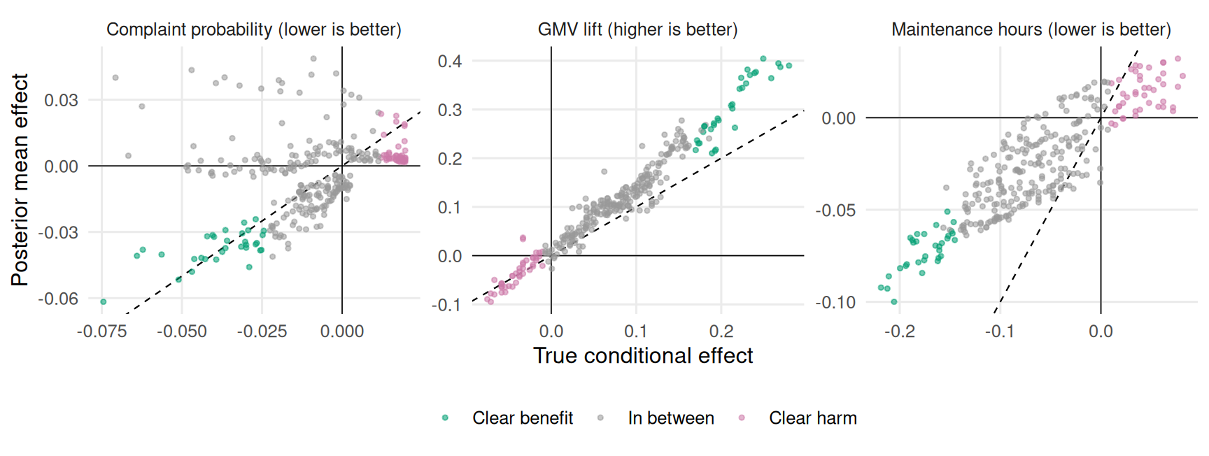
The effects are signed and opposing by construction: broad fulfilled sellers gain GMV, save time and attract fewer complaints, while narrow self-shipping sellers lose on all three. The `stopifnot()` confirms that **before** any model is fit, so that a model which fails to separate the two groups cannot be confused with a simulation that never separated them. The screen, fixed in advance: at eight weeks of exposure, GMV up at least 5%, maintenance hours down at least 10%, and complaint probability up by at most one point.
```{r multi-fit}
#| message: false
multi_budget <- list(joint = lb_budget(4), separate = lb_budget(2))
multi_key <- function(tag, budget) lb_key(tag, budget, LB_MODEL, digest::digest(md[c("y", "x", "z")]))
multi_conditions <- list(gmv = function(a) a >= log1p(MULTI_GMV_MIN),
                         seller_hours = function(a) a <= log1p(MULTI_HOURS_MAX),
                         complaint = function(a) a <= MULTI_COMPLAINT_MAX)
multi_cells <- matrix(FALSE, md$n, md$tt); multi_cells[, multi_col] <- TRUE
multi_export <- c("md", "multi_types", "multi_z_eval", "multi_col", "multi_conditions", "multi_cells",
                  "MULTI_GMV_MIN", "MULTI_HOURS_MAX", "MULTI_COMPLAINT_MAX")

multi_joint <- lb_artifact("multi_joint", multi_key("multi_joint", multi_budget$joint), export = c(multi_export, "multi_budget"),
  builder = function() {
    f <- do.call(longbet::longbet_multi,
                 c(list(y = md$y, x = md$x, z = md$z, t = seq_len(md$tt), outcome = multi_types,
                        sur = TRUE, sur_prior_var = 1, random_seed = 314159L), LB_MODEL, multi_budget$joint))
    p <- predict(f, x = md$x, z = multi_z_eval, t = seq_len(md$tt), summary_only = FALSE, random_seed = 271829L)
    obs <- predict(f, x = md$x, z = md$z, t = seq_len(md$tt), summary_only = TRUE, random_seed = 3L)
    list(draws = lapply(setNames(nm = names(multi_types)),
                        function(nm) matrix(effect_draws(p, nm)[, multi_col, ], nrow = md$n)),
         p_joint = as.vector(joint_prob(p, conditions = multi_conditions, cells = multi_cells)),
         att_obs = lapply(setNames(nm = names(multi_types)), function(nm) get_att(obs[nm])$att_full),
         correlation = outcome_correlation(f))
  })
multi_sep_draws <- lapply(setNames(nm = names(multi_types)), function(nm)
  lb_artifact(paste0("multi_", nm), multi_key(paste0("multi_", nm), multi_budget$separate), export = c(multi_export, "multi_budget"),
    builder = function() {
      f <- do.call(longbet::longbet,
                   c(list(y = md$y[[nm]], x = md$x, z = md$z, t = seq_len(md$tt),
                          outcome = unname(multi_types[[nm]]),
                          random_seed = 314160L + match(nm, names(multi_types))), LB_MODEL, multi_budget$separate))
      p <- predict(f, x = md$x, z = multi_z_eval, t = seq_len(md$tt), summary_only = FALSE, random_seed = 271830L)
      matrix(effect_draws(p)[, multi_col, ], nrow = md$n)
    }))
```
```{r multi-screen}
multi_draws <- multi_joint$draws
multi_layout <- chain_layout(multi_budget$joint$num_chains, multi_budget$joint$num_sweeps)
B <- list(multi_draws$gmv >= log1p(MULTI_GMV_MIN),
          multi_draws$seller_hours <= log1p(MULTI_HOURS_MAX),
          multi_draws$complaint <= MULTI_COMPLAINT_MAX)
multi_p_manual <- rowMeans(Reduce(`&`, B))
multi_p_marg <- lapply(B, rowMeans)
multi_p_product <- Reduce(`*`, multi_p_marg)
multi_p_separate <- rowMeans(multi_sep_draws$gmv >= log1p(MULTI_GMV_MIN)) *
  rowMeans(multi_sep_draws$seller_hours <= log1p(MULTI_HOURS_MAX)) *
  rowMeans(multi_sep_draws$complaint <= MULTI_COMPLAINT_MAX)
stopifnot(max(abs(multi_joint$p_joint - multi_p_manual)) < 1e-10,
          all(multi_p_manual >= pmax(0, Reduce(`+`, multi_p_marg) - 2) - 1e-12),
          all(multi_p_manual <= do.call(pmin, multi_p_marg) + 1e-12))
multi_truth_event <- multi_truth$gmv >= MULTI_GMV_MIN & multi_truth$seller_hours <= MULTI_HOURS_MAX &
  multi_truth$complaint <= MULTI_COMPLAINT_MAX
multi_est <- lapply(setNames(nm = names(multi_types)), function(nm)
  if (nm == "complaint") rowMeans(multi_draws[[nm]]) else rowMeans(expm1(multi_draws[[nm]])))
multi_region <- factor(ifelse(multi_good, "Clear benefit", ifelse(multi_bad, "Clear harm", "In between")),
                       levels = c("Clear benefit", "In between", "Clear harm"))
```
`effect_draws()` returns each outcome on the scale to reason on: the supplied log scale for the continuous outcomes, so a draw becomes a proportional change through $e^{\tau}-1$ per draw, and for the binary outcome the probability difference $\Phi(\mu_0+\tau)-\Phi(\mu_0)$ computed from the same draw. `joint_prob()` evaluates one predicate per outcome on the aligned draws. The `stopifnot()` checks it against a manual calculation and against the Fréchet bounds, seller by seller.
```{r multi-diagnostics}
multi_diag <- bind_rows(
  map_dfr(names(multi_types), function(nm)
    diagnose_draws(multi_joint$att_obs[[nm]], multi_layout, paste0("Average effect: ", nm))$summary),
  map_dfr(names(multi_types), function(nm)
    diagnose_draws(rbind(colMeans(multi_draws[[nm]][multi_good, ]), colMeans(multi_draws[[nm]][multi_bad, ])),
                   multi_layout, sprintf("Region means: %s", nm))$summary),
  map_dfr(names(multi_types), function(nm)
    diagnose_draws(multi_draws[[nm]], multi_layout, sprintf("Seller effects: %s", nm))$summary),
  diagnose_draws(1.0 * Reduce(`&`, B)[multi_p_manual > 0 & multi_p_manual < 1, , drop = FALSE], multi_layout,
                 sprintf("Joint-screen indicators with 0 < P < 1 (%d sellers)",
                         sum(multi_p_manual > 0 & multi_p_manual < 1)))$summary)
kable(multi_diag %>% select(-ok), digits = 3,
      caption = "Sampling checks for the joint fit, from each outcome's average effect down to every seller's screen indicator.")
```
```{r fig-multi-recovery}
#| fig-cap: "Known against estimated effect at eight weeks of exposure, by outcome. Colour marks two groups defined from the covariates; the model was never told the grouping. Beneficial is up for GMV and down for the other two."
#| fig-alt: "Three scatter panels along dashed diagonals. Green points sit in the beneficial quadrant of each panel and pink points in the opposite one, with the model's means tracking the truth in both."
#| fig-width: 9
#| fig-height: 3.4
multi_labels <- c(gmv = "GMV lift (higher is better)",
                  seller_hours = "Maintenance hours (lower is better)",
                  complaint = "Complaint probability (lower is better)")
map_dfr(names(multi_types), function(nm)
  tibble(outcome = multi_labels[[nm]], truth = multi_truth[[nm]], est = multi_est[[nm]], region = multi_region)) %>%
  ggplot(aes(truth, est, colour = region)) +
  geom_hline(yintercept = 0, linewidth = 0.3) + geom_vline(xintercept = 0, linewidth = 0.3) +
  geom_abline(linetype = "dashed", linewidth = 0.4) + geom_point(alpha = 0.55, size = 0.9) +
  facet_wrap(~ outcome, scales = "free") +
  scale_colour_manual(values = c("Clear benefit" = "#009E73", "In between" = "#999999",
                                 "Clear harm" = "#CC79A7")) +
  labs(x = "True conditional effect", y = "Posterior mean effect", colour = NULL) +
  theme(legend.position = "bottom", panel.grid.minor = element_blank())
```
```{r multi-tables}
tibble(Group = factor(paste(ifelse(md$listings >= 50, "Broad", "Narrow"),
                            ifelse(md$fulfilled == 1, "fulfilled", "self-ship"))),
       truth = multi_truth_event, joint = multi_joint$p_joint,
       prod_same = multi_p_product, prod_sep = multi_p_separate) %>%
  group_by(Group) %>%
  summarise(Sellers = n(), `True fraction` = mean(truth), `Joint fit` = mean(joint),
            `Same-fit product` = mean(prod_same), `Separate-fit product` = mean(prod_sep), .groups = "drop") %>%
  kable(digits = 3, caption = "The three-condition screen at eight weeks, by descriptive group: the expected fraction of sellers in each group that qualify.")
kable(multi_joint$correlation, digits = 3,
      caption = "Fitted innovation correlation across outcomes. The generating values were 0.60 for GMV with hours, 0.45 for GMV with the complaint latent, and 0.35 for hours with that latent.")
```
The joint fit recovers the residual correlation structure, separates the two signed regions on all three outcomes, and produces a per-seller probability that all three conditions hold together. The mean absolute difference between the joint probability and the product of the same fit's marginals is `r sprintf("%.3f", mean(abs(multi_joint$p_joint - multi_p_product)))`, with a largest gap of `r sprintf("%.3f", max(abs(multi_joint$p_joint - multi_p_product)))`: on this panel the dependence is modest, and the way to know that is to compute it rather than assume it.
What the joint model gives, and no product of separate fits can, is a distribution over **combinations** of effects. Any screen that involves more than one outcome at once, any trade-off rule, any "improve revenue without hurting complaints" constraint, is one line on the aligned draws.
## Conclusion
Dynamic effects become decisions through explicit assumptions: a baseline, a horizon, and a rule. Posterior draws carry the dependence between sellers, between periods and between outcomes through all of it, so the totals, the rankings and the joint screens come out of the same object that produced the average effect.
The **[next chapter](longbet_did.qmd)** puts the model side by side with the modern difference-in-differences estimators, and **[the one after](longbet_extensions.qmd)** takes it past the study window and into panels where nobody randomized adoption.