25  Ordinal Regression with BART and the Cloglog Link

25.1 Ordinal Outcomes in Business

Many of the outcomes we care about most in industry are ordered, but not numeric. Customer satisfaction is measured on a five-point Likert scale (one to five stars), Net Promoter Score (NPS) responses fall into detractor, passive, and promoter buckets, credit files are graded, and support tickets are triaged into severity tiers. While practitioners often treat these ratings as continuous numbers by averaging them, doing so imposes an unverifiable cardinal scale that assumes equal distances between categories and can produce severe distortions (Liddell and Kruschke (2018)). Rather than modeling raw scores with linear regression, standard Bayesian models for ordinal data rely on ordered probit and ordered logit (cumulative-link) models. These are a good starting point, but they carry two assumptions that are easy to overlook and frequently wrong:

1. Linearity and additivity. Predictors are assumed to impact a latent scale linearly, with no interactions unless we hand-specify them. For example, if a product change delights power users but frustrates newcomers, a linear model averages these out, reporting a misleading effect that describes neither group.
2. Ordered cutpoints in Gibbs sampling. Cumulative-link models rely on estimating thresholds (\(c_1 < \dots < c_{K-1}\)) that must remain strictly ordered. While Hamiltonian Monte Carlo (e.g., in Stan) handles ordered cutpoints in parametric models via monotonic transformations, Gibbs samplers—the standard engine for tree ensembles like BART—struggle with strong posterior dependencies among constrained cutpoints, which significantly degrades MCMC mixing and slows down convergence (Cowles (1996)).

In previous chapters, we saw how BART (Chipman et al. (2010)) relaxes the first assumption for continuous outcomes, discovering non-linearities and interactions on its own. This chapter extends that flexibility to ordinal outcomes, utilizing the framework from Alam and Linero (2025) to eliminate the second assumption as well.

25.2 The Cloglog Link and PHOBART

The fix starts with the link function. Instead of probit or logit, we use the complementary log-log (cloglog) link, \[ g(p) = \log\{-\log(1 - p)\}. \] It is the only link under which the two standard formulations of ordinal regression, cumulative-link and continuation-ratio, coincide (Läärä and Matthews (1985)). For an outcome with \(K\) ordered categories \(Y_i \in \{1, \dots, K\}\), Alam and Linero (2025) write the model in cumulative form: \[ \text{cloglog}(\Pr(Y_i \le k \mid X_i = x)) = c_k + \lambda(x), \] or equivalently in discrete proportional-hazards form, \[ \Pr(Y_i > k \mid X_i = x) = \{S_0(k)\}^{e^{+\lambda(x)}}, \] where \(S_0(k) = \exp(-e^{c_k})\) and \(\lambda(x)\) is assigned a BART sum-of-trees prior. Under this \(+ \lambda(x)\) convention, a larger \(\lambda(x)\) increases \(\Pr(Y_i \le k)\), shifting probability mass toward lower rating categories (worse outcomes). This yields a proportional hazards ordinal BART model (PHOBART).

It is helpful to separate the distinct roles of the link function and the tree ensemble: the cloglog link buys computation (unconstrained cutpoints and conjugate Gibbs updates), while BART’s sum-of-trees prior \(\lambda(x)\) buys flexibility (discovering non-linear threshold effects and subgroup heterogeneity across covariates \(X\)).

PHOBART resolves the cutpoint constraint issue that typically impedes Gibbs sampling in ordinal models. The strictly ordered cutpoints \(c_k\) are reparameterized through unconstrained parameters \(\gamma_j \in \mathbb{R}\) via: \[ c_k = \log \sum_{j \le k} e^{\gamma_j}, \qquad k = 1, \dots, K-1. \] Because the exponential is strictly positive, the ordering \(c_1 < c_2 < \dots < c_{K-1}\) holds by construction. Furthermore, because the inverse cloglog link is the CDF of an exponential distribution, augmenting each observation with a truncated-exponential latent variable allows the sampler to update the unconstrained parameters and the tree ensemble using standard conjugate and Gibbs updates. While the sampler works on the unconstrained scale, the package returns the transformed cutpoints \(c_k\).

Under suitable Hölder smoothness and sparsity conditions on the latent regression function \(\lambda(x)\), Alam and Linero (2025) prove that PHOBART achieves minimax-optimal posterior contraction rates (up to logarithmic factors), guaranteeing that the posterior concentrates around the true data-generating process at the optimal statistical rate.

The same latent-exponential machinery unifies ordinal, survival, and density regression under one framework. In the practical example below, our code targets stochtree version 0.4.5 (and stochtree >= 0.4.5).

25.3 A Business Example: A Feature Change and Customer Satisfaction

Suppose we roll out a product change and measure its effect on a one-to-five satisfaction rating. Our concern is heterogeneity: we suspect the change helps some customers and hurts others depending on how engaged they were to begin with. If we are right, a linear ordered probit will average those opposing effects into something misleading, and we could ship (or kill) the feature for the wrong reason.

To see this cleanly, we simulate data where we know the truth. Let x1 be a centered engagement score and t the feature flag. The latent satisfaction z is defined as \[ z = 1.5 \sin\!\left(\frac{\pi\, x_1}{2}\right) + \tau(x_1)\, t + \epsilon, \qquad \epsilon \sim \mathcal{N}(0, 0.8^2), \] where the feature’s effect \(\tau(x_1)\) is \(+1.5\) for engaged customers (\(x_1 > 0\)) and \(-1.0\) for less-engaged ones (\(x_1 \le 0\)). This construction induces both a non-linear baseline effect through the sine function and heterogeneous treatment effects whose sign depends on \(x_1\).

The observed ordinal outcome is generated by discretizing \(z\) into a five-point Likert scale using fixed thresholds. Because treatment \(t\) is assigned completely at random (\(t \sim \text{Bernoulli}(0.5)\)) independent of \(x_1\), causal identification (unconfoundedness and overlap) holds by design. This isolates the comparison entirely to the functional form: whether each model can accurately discover the non-linear response surface and subgroup heterogeneity. The latent noise is Gaussian, which favors the probit benchmark in terms of link specification.

library(ggplot2)
library(dplyr)
library(tidyr)
library(stochtree)
library(brms)
library(coda)
library(knitr)

set.seed(1982)
N <- 2500

fake_data <- tibble(
  x1 = runif(N, -2, 2),
  t  = sample(c(0, 1), N, replace = TRUE)
) %>%
  mutate(
    f_x    = 1.5 * sin(pi * x1 / 2),
    tau_x  = ifelse(x1 > 0, 1.5, -1.0),
    z_true = f_x + tau_x * t + rnorm(N, 0, 0.8),
    y = case_when(
      z_true <  -1.5 ~ 1,
      z_true <  -0.5 ~ 2,
      z_true <   0.5 ~ 3,
      z_true <   1.5 ~ 4,
      TRUE           ~ 5
    )
  )

# Verify all five rating categories are well-populated
table(fake_data$y)

  1   2   3   4   5 
622 459 373 355 691 

We then compute the true population effect of the feature on each rating level by integrating over the counterfactuals (feature off vs. feature on) for every customer.

truth_ate <- fake_data %>%
  mutate(z0 = f_x, z1 = f_x + tau_x) %>%
  mutate(
    p0_1 = pnorm(-1.5, z0, 0.8),
    p0_2 = pnorm(-0.5, z0, 0.8) - pnorm(-1.5, z0, 0.8),
    p0_3 = pnorm( 0.5, z0, 0.8) - pnorm(-0.5, z0, 0.8),
    p0_4 = pnorm( 1.5, z0, 0.8) - pnorm( 0.5, z0, 0.8),
    p0_5 = 1 - pnorm(1.5, z0, 0.8),
    p1_1 = pnorm(-1.5, z1, 0.8),
    p1_2 = pnorm(-0.5, z1, 0.8) - pnorm(-1.5, z1, 0.8),
    p1_3 = pnorm( 0.5, z1, 0.8) - pnorm(-0.5, z1, 0.8),
    p1_4 = pnorm( 1.5, z1, 0.8) - pnorm( 0.5, z1, 0.8),
    p1_5 = 1 - pnorm(1.5, z1, 0.8)
  ) %>%
  summarise(across(starts_with("p0_") | starts_with("p1_"), mean)) %>%
  pivot_longer(everything(), names_to = c("group", "y"), names_sep = "_") %>%
  pivot_wider(names_from = group, values_from = value) %>%
  mutate(y = as.integer(y), tau = p1 - p0)

kable(
  truth_ate,
  digits = 3,
  col.names = c("Rating (y)", "P(Y=y | t=0)", "P(Y=y | t=1)", "True ATE (tau)")
)

Rating (y)	P(Y=y | t=0)	P(Y=y | t=1)	True ATE (tau)
1	0.148	0.357	0.209
2	0.238	0.129	-0.109
3	0.247	0.037	-0.211
4	0.226	0.066	-0.160
5	0.141	0.412	0.270

BART Model Fitting (PHOBART)

We fit the PHOBART model using stochtree::bart() with an OutcomeModel specifying outcome = "ordinal" and link = "cloglog" inside general_params. We also configure key hyperparameters:

• sample_sigma2_global = FALSE: Ordinal outcomes do not have a free Gaussian residual variance \(\sigma^2\) because scale is fixed by the link function.
• random_seed = 2025: In stochtree, MCMC sampling randomness is controlled via random_seed inside general_params rather than base R’s set.seed().
• mean_forest_params = list(num_trees = 50, sample_sigma2_leaf = FALSE): Configures 50 trees and fixes the leaf shrinkage parameter at its prior default rather than sampling it adaptively.
• num_gfr = 0: Runs standard MCMC sampling from initialization.

We run a single MCMC chain here for illustration and monitor ESS and trace plots; in production settings, one can set num_chains in stochtree::bart() to assess convergence diagnostics such as \(\hat{R}\) across multiple independent chains alongside ESS.

X_train <- fake_data %>% select(x1, t) %>% as.matrix()
y_train <- fake_data$y

X0 <- X_train; X0[, "t"] <- 0
X1 <- X_train; X1[, "t"] <- 1

phobart <- bart(
  X_train = X_train,
  y_train = y_train,
  num_gfr = 0,
  num_burnin = 1000,
  num_mcmc   = 1000,
  general_params = list(
    sample_sigma2_global = FALSE,
    random_seed = 2025,
    outcome_model = OutcomeModel(outcome = "ordinal", link = "cloglog")
  ),
  mean_forest_params = list(num_trees = 50, sample_sigma2_leaf = FALSE)
)

Checking convergence

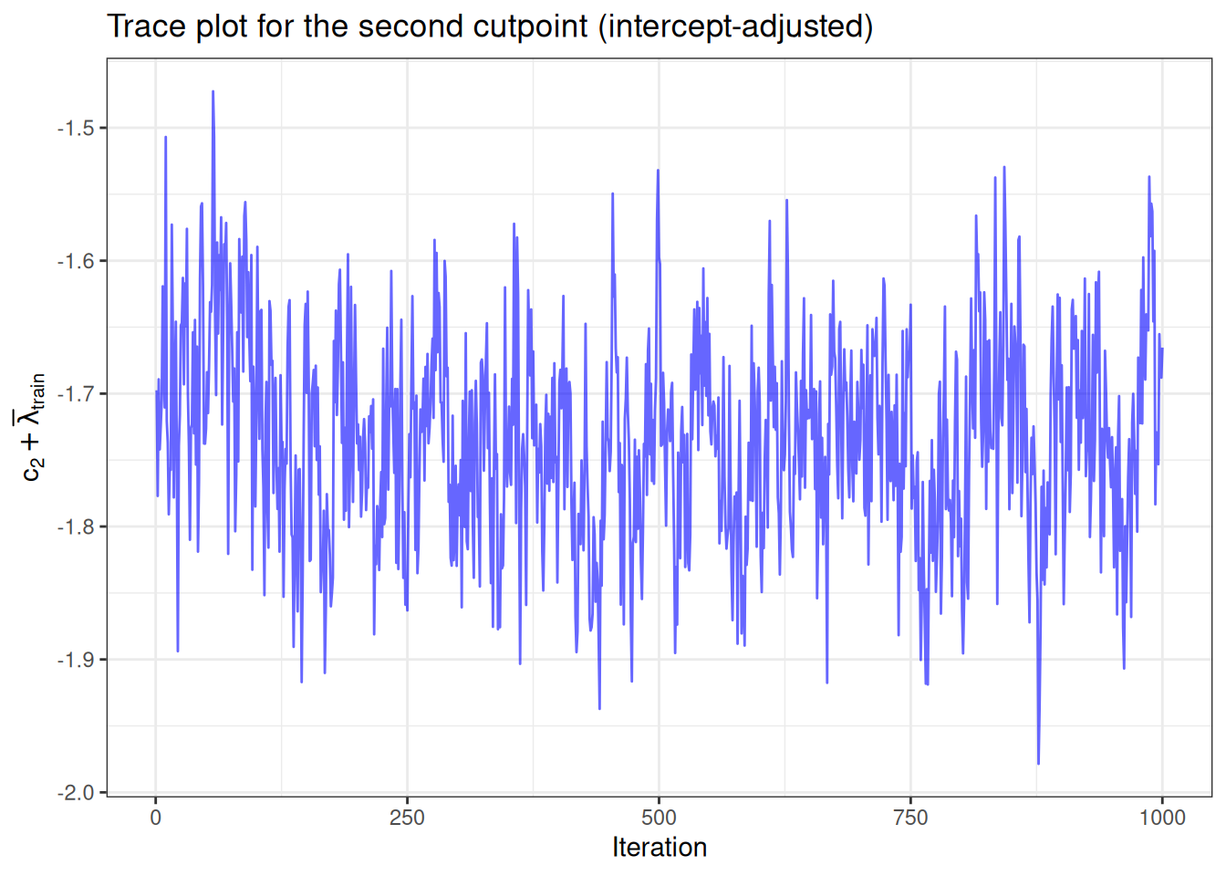
Before trusting the estimates, we check that the MCMC sampler has mixed well. Cutpoint draws are extracted via extractParameter(phobart, "cloglog_cutpoints"), returning a matrix of shape \((K-1, S)\) containing draws of \(c_k\).

Because the tree ensemble \(\lambda(x)\) can absorb an arbitrary global shift (an implicit intercept), raw cutpoint draws \(c_k\) and the forest predictions share a non-identifiable additive constant. If unadjusted, raw cutpoints can drift even in a well-converged chain, yielding a misleadingly low Effective Sample Size (ESS). To evaluate convergence on a strictly identified quantity, we shift the cutpoints by the per-sample mean of the training predictions, \(\bar{\lambda}_{\text{train}} = \frac{1}{N}\sum_{i=1}^N \lambda(X_i)\), tracing \(c_2 + \bar{\lambda}_{\text{train}}\). (Note that this shift automatically cancels when computing counterfactual contrast probabilities.)

cutpoint_draws <- extractParameter(phobart, "cloglog_cutpoints")
lambda_train   <- predict(
  phobart, X_train, scale = "linear", terms = "y_hat", type = "posterior"
)

# Shift cutpoints by the mean training latent prediction
adj_c2 <- cutpoint_draws[2, ] + colMeans(lambda_train)

tibble(
  iteration = seq_along(adj_c2),
  c2_adj    = adj_c2
) %>%
  ggplot(aes(iteration, c2_adj)) +
  geom_line(color = "blue", alpha = 0.6) +
  labs(
    title = "Trace plot for the second cutpoint (intercept-adjusted)",
    x = "Iteration",
    y = expression(c[2] + bar(lambda)[train])
  ) +
  theme_bw()

cat("ESS for adjusted c_2:", round(effectiveSize(adj_c2), 1), "\n")

ESS for adjusted c_2: 104.6 

The trace looks stationary with no drift or sticking. An ESS of approximately 105 from 1,000 posterior draws (~10% efficiency) is adequate for exploring central tendencies and median treatment effects, though estimating extreme tail intervals with high precision in production typically calls for longer sampling runs where \(\text{ESS} \gtrsim 400\) per tail quantity is standard. In practice, you would inspect the remaining thresholds and tree ensemble predictions similarly.

Turning the posterior into category probabilities

Instead of manually evaluating the link algebra, stochtree provides a direct accessor: predict(..., scale = "probability", terms = "y_hat", type = "posterior") returns an array of dimension \((\text{observations}, \text{categories}, \text{samples})\). Averaging over observations yields the population-level category probabilities for each posterior draw.

# Predict category probabilities: returns (observations, categories, samples)
probs0 <- predict(
  phobart, X0, scale = "probability", terms = "y_hat", type = "posterior"
)
probs1 <- predict(
  phobart, X1, scale = "probability", terms = "y_hat", type = "posterior"
)

# Average over observations to get population category probabilities per sample
pop0_phobart <- t(apply(probs0, c(2, 3), mean)) # samples x categories
pop1_phobart <- t(apply(probs1, c(2, 3), mean))

tau_phobart <- as_tibble(
  pop1_phobart - pop0_phobart,
  .name_repair = ~ paste0("V", seq_along(.x))
) %>%
  mutate(draw = row_number()) %>%
  pivot_longer(-draw, names_to = "y", values_to = "tau") %>%
  mutate(y = as.integer(sub("V", "", y)))

Benchmark: linear ordered probit

To benchmark our approach, we fit a Bayesian linear ordered probit model with brms, to see how it performs when the true relationship is non-linear and includes interactions.

dir.create("cache", showWarnings = FALSE)

probit_lm <- brm(
  y ~ x1 + t,
  data    = fake_data %>% mutate(y = ordered(y)),
  family  = cumulative("probit"),
  chains  = 4, cores = 4, iter = 2000, refresh = 0,
  seed    = 2025,
  file    = "cache/probit_lm"
)

# posterior_epred returns draws x observations x categories for ordinal families
ep0 <- posterior_epred(
  probit_lm,
  newdata = fake_data %>% mutate(t = 0, y = ordered(y))
)
ep1 <- posterior_epred(
  probit_lm,
  newdata = fake_data %>% mutate(t = 1, y = ordered(y))
)

pop0_probit <- apply(ep0, c(1, 3), mean)   # draws x categories
pop1_probit <- apply(ep1, c(1, 3), mean)

tau_probit <- as_tibble(
  pop1_probit - pop0_probit,
  .name_repair = ~ paste0("V", seq_along(.x))
) %>%
  mutate(draw = row_number()) %>%
  pivot_longer(-draw, names_to = "y", values_to = "tau") %>%
  mutate(y = as.integer(sub("V", "", y)))

Comparison of Average Treatment Effects

summ <- function(df, model) {
  df %>% group_by(y) %>%
    summarise(val  = median(tau),
              low  = quantile(tau, 0.025),
              high = quantile(tau, 0.975), .groups = "drop") %>%
    mutate(Model = model)
}

bind_rows(summ(tau_phobart, "PHOBART"), summ(tau_probit, "Linear Probit")) %>%
  ggplot(aes(factor(y), val, color = Model)) +
  geom_linerange(aes(ymin = low, ymax = high), linewidth = 1,
                 position = position_dodge(0.5)) +
  geom_point(size = 3, position = position_dodge(0.5)) +
  geom_point(data = truth_ate, aes(factor(y), tau, color = "Truth"),
             size = 4, shape = 4, stroke = 1.5, inherit.aes = FALSE) +
  geom_hline(yintercept = 0, linetype = "dashed", alpha = 0.5) +
  scale_color_manual(
    values = c(
      "PHOBART"       = "#0072B2",
      "Linear Probit" = "#D55E00",
      "Truth"         = "#000000"
    )
  ) +
  labs(
    title = "Effect of the feature on each rating level",
    subtitle = paste0(
      "The linear model averages away the sign-flipping heterogeneity"
    ),
    x = "Rating (1–5)",
    y = "Change in probability"
  ) +
  theme_bw() + theme(legend.position = "bottom")

Figure 25.1: Comparison of average treatment effect estimates across models against the ground truth.

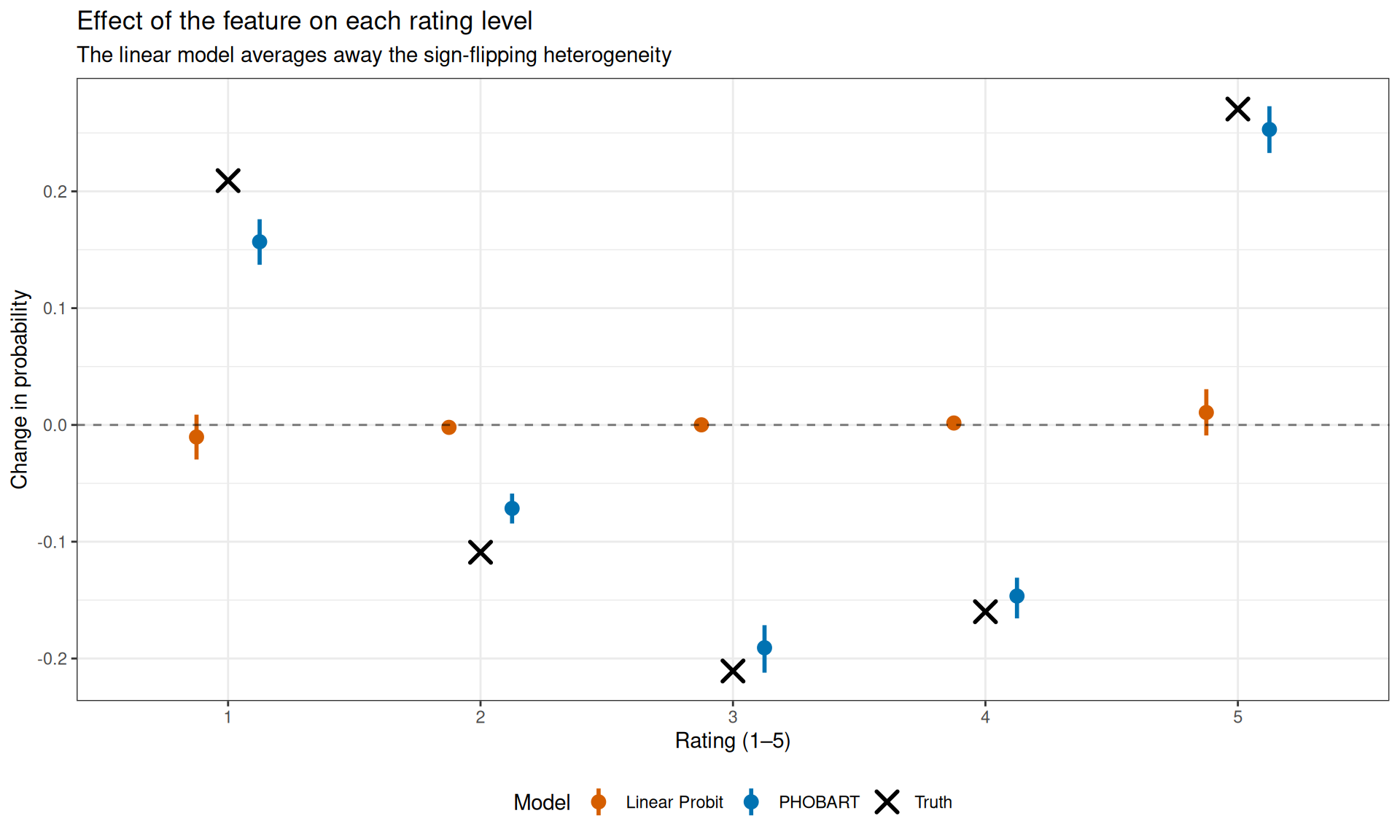
As shown in Figure 25.1, the two models tell radically different stories about how the product change impacts customer experience:

• Rating 1 (1 Star): The linear probit estimates a small decrease in 1-star ratings. The true latent shift averages to \(0.5(1.5) + 0.5(-1.0) = 0.25\). On the identified probit scale (where the residual variance denominator is inflated by the unmodeled sine variation), the linear model estimates a small positive treatment coefficient (\(\hat{\beta}_t \approx 0.24\)), forcing the modeled probability of the lowest category to fall (\(\approx -0.01\)). In reality, the harmed subgroup (\(x_1 \le 0\)) is pushed below the \(-1.5\) threshold, causing 1-star reviews to increase by 20.9 points (\(+0.209\)). The linear model commits a dangerous sign error on the company’s most dissatisfied customers.
• Ratings 2, 3, and 4: Under the true data-generating process, probability mass drains out of the middle ratings as customers polarize toward the extremes. The linear probit predicts negligible changes across these tiers, missing the hollowed-out middle.
• Rating 5 (5 Stars): The linear probit points in the right direction at the top of the scale (\(\approx +0.01\)), but its estimate is indistinguishable from zero (its 95% credible interval crosses zero) and roughly 25× too small. In contrast, PHOBART captures the large positive surge in 5-star reviews (\(\approx +0.25\)) driven by delighted power users (\(x_1 > 0\)).
• Overall: PHOBART captures the qualitative U-shaped polarization that the linear model misses entirely. At the same time, notice that PHOBART’s 95% credible intervals are moderately shrunk toward zero relative to the ground truth. This attenuation stems from two factors: (1) tree shrinkage priors with 50 trees, and (2) link misspecification, as the true data-generating process uses a Gaussian location shift rather than an exact proportional-hazards cloglog link. Even under this link mismatch, PHOBART successfully recovers the correct directional dynamics across every category.

25.4 Why These Results Matter

In this data-generating process, the treatment effect is heterogeneous: it is positive for individuals with \(x_1 > 0\) and negative for those with \(x_1 \le 0\). A cumulative-link model with a single additive treatment coefficient is forced to represent this structure using a single global shift, which washes out opposing subgroup effects. (A parametric model with an explicit interaction term like y ~ x1 * t could in principle accommodate heterogeneity, but that requires the analyst to already know the exact interaction structure in advance—which is rarely possible in production.)

The linear model’s failure here is not subtle: it tells leadership that angry reviews are dropping when they are actually spiking. The PHOBART model correctly identifies both the non-linear baseline relationship between \(x_1\) and the outcome and the interaction between \(x_1\) and treatment. This is the practical payoff: when an intervention helps some customers and hurts others, only a flexible model reveals the trade-off.

Decision-Making Under Polarization: What to Do Monday Morning

The core business dynamic demonstrated here is customer polarization: the feature drives mass to both ends of the scale, creating 5-star advocates and 1-star detractors while hollowing out everything in between—including 4-star ratings, which fall by 16 points.

This polarization easily fools high-level executive dashboards. Looking only at summary metrics from the true population distribution, the average customer rating inches up by a negligible 0.07 stars (\(2.98 \to 3.05\)), and an NPS-style net score (\(4\text{--}5\) star ratings minus \(1\text{--}2\) star ratings) improves from \(-1.8\%\) to \(-0.8\%\). Yet under the hood, 1-star reviews surge from \(14.8\%\) to \(35.7\%\)—a \(2.4\times\) explosion in furious customers.

Because Bayesian models produce posterior draws across the full probability distribution, we can directly query the posterior for decision-relevant probabilities:

# Compute promoter and detractor comparisons
prob_prom_probit <- mean(
  (pop1_probit[, 4] + pop1_probit[, 5]) > (pop0_probit[, 4] + pop0_probit[, 5])
)
prob_detr_probit <- mean(pop1_probit[, 1] > pop0_probit[, 1])
prob_pol_probit  <- mean(
  ((pop1_probit[, 4] + pop1_probit[, 5]) >
   (pop0_probit[, 4] + pop0_probit[, 5])) &
  (pop1_probit[, 1] > pop0_probit[, 1])
)

prob_prom_phobart <- mean(
  (pop1_phobart[, 4] + pop1_phobart[, 5]) >
  (pop0_phobart[, 4] + pop0_phobart[, 5])
)
prob_detr_phobart <- mean(pop1_phobart[, 1] > pop0_phobart[, 1])
prob_pol_phobart  <- mean(
  ((pop1_phobart[, 4] + pop1_phobart[, 5]) >
   (pop0_phobart[, 4] + pop0_phobart[, 5])) &
  (pop1_phobart[, 1] > pop0_phobart[, 1])
)

fmt_pct <- function(p) {
  if (p >= 0.999) return(">99.9%")
  if (p <= 0.001) return("<0.1%")
  sprintf("%.1f%%", 100 * p)
}

decision_summary <- tibble(
  `Business Question` = c(
    "Pr(Top-box share [4–5 stars] increased)",
    "Pr(Bottom-box share [1 star] increased)",
    "Pr(Polarization: Both 1-star and top-box shares increased)"
  ),
  `Linear Probit` = c(
    fmt_pct(prob_prom_probit),
    fmt_pct(prob_detr_probit),
    fmt_pct(prob_pol_probit)
  ),
  `PHOBART` = c(
    fmt_pct(prob_prom_phobart),
    fmt_pct(prob_detr_phobart),
    fmt_pct(prob_pol_phobart)
  )
)

kable(
  decision_summary,
  col.names = c("Decision-Relevant Question", "Linear Probit", "PHOBART")
)

Decision-Relevant Question	Linear Probit	PHOBART
Pr(Top-box share [4–5 stars] increased)	85.2%	>99.9%
Pr(Bottom-box share [1 star] increased)	14.8%	>99.9%
Pr(Polarization: Both 1-star and top-box shares increased)	<0.1%	>99.9%

Note that while the polarization verdict is robust across reasonable bucketings (for instance, defining detractors as 1–2 stars still yields a \(+10.0\%\) increase), net summary scores remain sensitive to threshold choices (defining detractors as 1–3 stars flips the net effect to \(-11.0\%\)), highlighting the risk of collapsing ordinal distributions into single numbers.

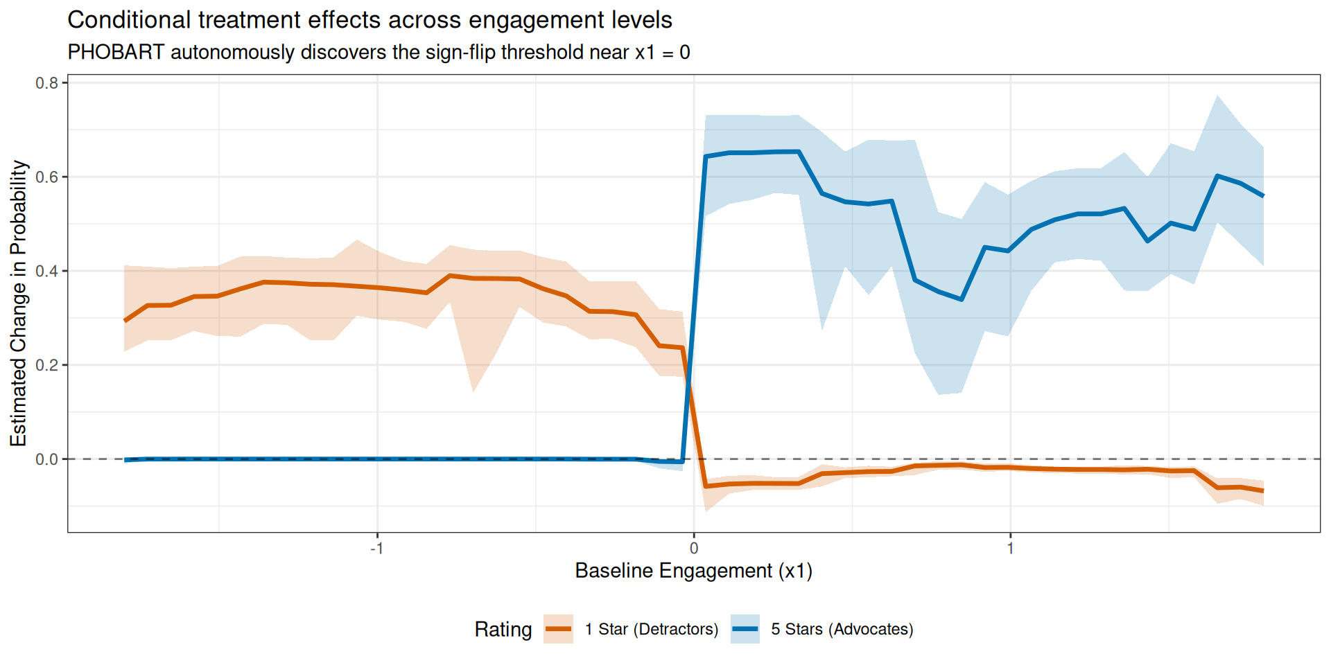
To justify concrete operational actions on Monday morning, we inspect how the treatment effect on extreme ratings varies across customer engagement levels \(x_1\):

x1_grid <- seq(-1.8, 1.8, length.out = 50)
grid0   <- cbind(x1 = x1_grid, t = 0)
grid1   <- cbind(x1 = x1_grid, t = 1)

g_p0 <- predict(
  phobart, grid0, scale = "probability", terms = "y_hat", type = "posterior"
)
g_p1 <- predict(
  phobart, grid1, scale = "probability", terms = "y_hat", type = "posterior"
)

tau1_grid <- g_p1[, 1, ] - g_p0[, 1, ]
tau5_grid <- g_p1[, 5, ] - g_p0[, 5, ]

df_het <- tibble(
  x1 = rep(x1_grid, 2),
  Rating = rep(
    c("1 Star (Detractors)", "5 Stars (Advocates)"),
    each = 50
  ),
  val  = c(apply(tau1_grid, 1, median), apply(tau5_grid, 1, median)),
  low  = c(apply(tau1_grid, 1, quantile, 0.025),
           apply(tau5_grid, 1, quantile, 0.025)),
  high = c(apply(tau1_grid, 1, quantile, 0.975),
           apply(tau5_grid, 1, quantile, 0.975))
)

ggplot(df_het, aes(x1, val, color = Rating, fill = Rating)) +
  geom_ribbon(aes(ymin = low, ymax = high), alpha = 0.2, color = NA) +
  geom_line(linewidth = 1.2) +
  geom_hline(yintercept = 0, linetype = "dashed", alpha = 0.5) +
  scale_color_manual(
    values = c(
      "1 Star (Detractors)" = "#D55E00",
      "5 Stars (Advocates)"  = "#0072B2"
    )
  ) +
  scale_fill_manual(
    values = c(
      "1 Star (Detractors)" = "#D55E00",
      "5 Stars (Advocates)"  = "#0072B2"
    )
  ) +
  labs(
    title = "Conditional treatment effects across engagement levels",
    subtitle = paste0(
      "PHOBART autonomously discovers the sign-flip threshold near x1 = 0"
    ),
    x = "Baseline Engagement (x1)",
    y = "Estimated Change in Probability"
  ) +
  theme_bw() + theme(legend.position = "bottom")

Figure 25.2: Estimated conditional treatment effect on 1-star and 5-star ratings across engagement levels under PHOBART.

As demonstrated in Figure 25.2, PHOBART autonomously discovers the inflection point near \(x_1 = 0\) without parametric guidance. This empowers leadership to make targeted, data-backed decisions:

1. Cohort-Gated Rollout: Ship the feature immediately to power users and highly engaged accounts (\(x_1 > 0\)), where 5-star reviews surge by 40–50 percentage points and negative sentiment is absent.
2. Product Redesign for Onboarding: Pause exposure for less-engaged customers (\(x_1 \le 0\)), where 1-star reviews spike by 30–40 points, iterating on simpler onboarding and UI guidance before re-testing.

Diagnosing Model Misfit Without Ground Truth

In real industry applications, analysts do not have access to ground truth benchmarks. How can a team detect that an additive model has failed?

1. Subgroup Calibration & Posterior Predictive Checks (PPCs): Bin the observed data by customer cohorts (such as \(x_1 \le 0\) vs. \(x_1 > 0\)) and compare observed proportions against the model’s posterior predictions. For treated customers with \(x_1 \le 0\), the empirical share of 1-star ratings is roughly \(50\%\), yet the linear probit predicts only \(\approx 13\%\). This glaring discrepancy immediately exposes model misspecification.
2. Model Comparison via Out-of-Sample Validation: Evaluating leave-one-out cross-validation (e.g., via loo) or predictive log-likelihood quickly flags that an additive model fails to capture systematic patterns across engagement deciles.

25.5 Conclusion

This example illustrates the practical value of a unified Bayesian nonparametric framework: it is easier to implement because it avoids cutpoint constraints, and more accurate because it adapts automatically to complex structure in the data.

The usual cautions apply. The causal reading rests on the standard assumptions, unconfoundedness and adequate overlap between treated and control units, which no model supplies on its own; when treatment is not randomized, including a propensity score as an additional covariate can mitigate regularization-induced confounding (Hahn et al. (2020)), though causal identification ultimately depends on unconfoundedness and adequate overlap. The proportional-hazards version assumes the covariate effect does not interact with the rating level; the non-proportional variant (NPHOBART) relaxes this at some computational cost. Alam and Linero (2025) develop PHOBART and NPHOBART for ordinal regression and note that sharing forests, in the spirit of Hahn et al. (2020), is a natural route to richer causal estimation.

TipLearn more

For the theoretical framework, minimax posterior contraction proofs, and extensions to non-proportional hazards ordinal regression (NPHOBART), see Alam and Linero (2025), A unified Bayesian nonparametric framework for ordinal, survival, and density regression using the complementary log-log link (arXiv:2502.00606).

25.6 Appendix: Session Information

sessionInfo()

R version 4.6.1 (2026-06-24)
Platform: x86_64-pc-linux-gnu
Running under: Ubuntu 24.04.4 LTS

Matrix products: default
BLAS:   /usr/lib/x86_64-linux-gnu/openblas-pthread/libblas.so.3 
LAPACK: /usr/lib/x86_64-linux-gnu/openblas-pthread/libopenblasp-r0.3.26.so;  LAPACK version 3.12.0

locale:
 [1] LC_CTYPE=C.UTF-8       LC_NUMERIC=C           LC_TIME=C.UTF-8       
 [4] LC_COLLATE=C.UTF-8     LC_MONETARY=C.UTF-8    LC_MESSAGES=C.UTF-8   
 [7] LC_PAPER=C.UTF-8       LC_NAME=C              LC_ADDRESS=C          
[10] LC_TELEPHONE=C         LC_MEASUREMENT=C.UTF-8 LC_IDENTIFICATION=C   

time zone: UTC
tzcode source: system (glibc)

attached base packages:
[1] stats     graphics  grDevices utils     datasets  methods   base     

other attached packages:
[1] knitr_1.51      coda_0.19-4.1   brms_2.23.0     Rcpp_1.1.2     
[5] stochtree_0.4.5 tidyr_1.3.2     dplyr_1.2.1     ggplot2_4.0.3  

loaded via a namespace (and not attached):
 [1] tensorA_0.36.2.1     bridgesampling_1.2-1 generics_0.1.4      
 [4] stringi_1.8.9        lattice_0.22-9       digest_0.6.39       
 [7] magrittr_2.0.5       evaluate_1.0.5       grid_4.6.1          
[10] RColorBrewer_1.1-3   mvtnorm_1.4-2        fastmap_1.2.0       
[13] jsonlite_2.0.0       Matrix_1.7-5         processx_3.9.0      
[16] pkgbuild_1.4.8       backports_1.5.1      ps_1.9.3            
[19] gridExtra_2.3.1      Brobdingnag_1.2-9    purrr_1.2.2         
[22] QuickJSR_1.10.0      scales_1.4.0         codetools_0.2-20    
[25] abind_1.4-8          cli_3.6.6            rlang_1.3.0         
[28] withr_3.0.3          yaml_2.3.12          otel_0.2.0          
[31] StanHeaders_2.32.10  inline_0.3.21        rstan_2.32.7        
[34] tools_4.6.1          parallel_4.6.1       rstantools_2.7.0    
[37] checkmate_2.3.4      vctrs_0.7.3          posterior_1.7.0     
[40] R6_2.6.1             stats4_4.6.1         matrixStats_1.5.0   
[43] lifecycle_1.0.5      stringr_1.6.0        htmlwidgets_1.6.4   
[46] callr_3.8.0          pkgconfig_2.0.3      RcppParallel_6.2.0  
[49] pillar_1.11.1        gtable_0.3.6         loo_2.10.1          
[52] glue_1.8.1           xfun_0.60            tibble_3.3.1        
[55] tidyselect_1.2.1     farver_2.1.2         bayesplot_1.15.0    
[58] htmltools_0.5.9      nlme_3.1-169         labeling_0.4.3      
[61] rmarkdown_2.31       compiler_4.6.1       S7_0.2.2            
[64] distributional_0.8.1

Alam, Entejar, and Antonio R Linero. 2025. “A Unified Bayesian Nonparametric Framework for Ordinal, Survival, and Density Regression Using the Complementary Log-Log Link.” arXiv Preprint arXiv:2502.00606.

Chipman, Hugh A., Edward I. George, and Robert E. McCulloch. 2010. “BART: Bayesian additive regression trees.” The Annals of Applied Statistics 4 (1): 266–98. https://doi.org/10.1214/09-AOAS285.

Cowles, Mary Kathryn. 1996. “Accelerating Monte Carlo Markov Chain Convergence for Cumulative-Link Generalized Linear Models.” Statistics and Computing 6 (2): 101–11. https://doi.org/10.1007/bf00162520.

Hahn, P Richard, Jared S Murray, and Carlos M Carvalho. 2020. “Bayesian Regression Tree Models for Causal Inference: Regularization, Confounding, and Heterogeneous Effects (with Discussion).” Bayesian Analysis 15 (3): 965–1056. https://doi.org/10.1214/19-BA1195.

Läärä, Esa, and John N S Matthews. 1985. “The Equivalence of Two Models for Ordinal Data.” Biometrika 72 (1): 206–7. https://doi.org/10.1093/biomet/72.1.206.

Liddell, Torrin M, and John K Kruschke. 2018. “Analyzing Ordinal Data with Metric Models: What Could Possibly Go Wrong?” Journal of Experimental Social Psychology 79: 328–48. https://doi.org/10.1016/j.jesp.2018.08.009.