library(longbet)
library(dplyr)
library(tidyr)
library(tibble)
library(ggplot2)
library(purrr)
library(knitr)
library(did)
library(fixest)
library(didimputation)
library(bacondecomp)
library(fect)

source("R/longbet-common.R")
source("R/longbet-sim.R")
source("R/longbet-artifacts.R")
verify_longbet_environment()
theme_set(theme_minimal(base_size = 12))

DID_PAL <- c(Truth = "#000000", `TWFE event study` = "#d95f02",
             `Callaway & Sant'Anna` = "#7570b3", `Callaway & Sant'Anna, covariates` = "#a6761d",
             `Sun & Abraham` = "#e7298a", `Borusyak, Jaravel & Spiess` = "#e6ab02",
`Interactive fixed effects` = "#1b9e77", LongBet = "#0072B2")27 LongBet and Modern Difference-in-Differences
NotePart of the LongBet sequence
This chapter sits between LongBet: From Effects to Decisions and LongBet: Forecasting and Observational Panels. It is self-contained: the panels here are new, small, and built to isolate one question at a time. The last of them reproduces the simulation design of Wang et al. (2026), so its results can be read next to the paper’s tables.
27.1 The Question a Reviewer Will Ask
Present a panel model of a staggered rollout and someone will ask why you did not run the estimator from the econometrics literature. It is a fair question with a precise answer, and this chapter gives it by running both on the same data.
The modern staggered difference-in-differences toolkit exists because the canonical two-way fixed effects (TWFE) event study breaks under staggered adoption. Goodman-Bacon (2021) showed that its coefficient is a weighted average of all the two-by-two comparisons available in the panel, including forbidden ones that use already-treated units as controls for later-treated units. When effects grow with exposure, those comparisons subtract a rising treated trend and can flip the sign of the answer. The repairs are well known: Callaway and Sant’Anna (2021) estimate group-time effects against never-treated or not-yet-treated units and aggregate afterwards, optionally conditioning on covariates through a doubly robust score; Sun and Abraham (2021) build an interaction-weighted event study; and Borusyak et al. (2024) impute untreated potential outcomes from a model fitted on untreated cells only. A different tradition relaxes parallel trends instead of conditioning on covariates: interactive fixed effects, or the generalized synthetic control of Xu (2017), fits a low-rank factor structure to the untreated panel and imputes from it.
Those estimators are excellent at what they do. This chapter’s claim is narrow and, I think, useful: on a panel they were built for, LongBet matches them; on a panel where the effect varies across units, it answers a question they are not built to answer; and on a panel where untreated trends diverge with the covariates, it adjusts for something the linear covariate adjustment cannot represent.
# One long-format panel per simulation, in the shape the econometric packages expect. A simulator
# may supply `x_did`, a data frame in which an unordered factor stays a factor; the model matrix
# `x` handed to LongBet carries the same information as dummies.
panel_long <- function(sim) {
  n <- nrow(sim$y)
  df <- expand.grid(id = seq_len(n), time = sim$tg)
  df <- df[order(df$id, df$time), ]
  df$y <- as.vector(t(sim$y))
  df$treat <- as.vector(t(sim$z))
  df$first_treat <- sim$adopt[df$id]
  df$first_treat_did <- ifelse(is.finite(df$first_treat), df$first_treat, 0)
  df$rel_time <- ifelse(df$first_treat_did == 0, -1000, df$time - df$first_treat)
  xs <- if (!is.null(sim$x_did)) sim$x_did else as.data.frame(sim$x)
  for (j in names(xs)) df[[j]] <- xs[df$id, j]
  df
}

# Each estimator's event-study curve, aligned on exposure S = event time + 1 so that every
# method reports the same quantity on the same axis. Intervals are pointwise 95% throughout.
# `xformla` adds a covariate-adjusted Callaway-Sant'Anna run; `ife` adds interactive fixed
# effects, whose factor dimension is chosen by cross-validation.
did_event_curves <- function(df, max_s, xformla = NULL, ife = FALSE, seed = 1) {
  set.seed(seed)
  align <- function(event_time, est, lo, hi) {
    m <- match(seq_len(max_s) - 1, event_time)
    tibble(s = seq_len(max_s), estimate = est[m], lower = lo[m], upper = hi[m])
  }
  tw <- feols(y ~ i(rel_time, ref = c(-1, -1000)) | id + time, data = df)
  tw_ct <- as.data.frame(summary(tw)$coeftable)
  tw_ev <- suppressWarnings(as.numeric(sub(".*::", "", rownames(tw_ct))))
  cs_curve <- function(xf, label) {
    cs <- aggte(att_gt(yname = "y", tname = "time", idname = "id", gname = "first_treat_did",
                       xformla = xf, data = df, control_group = "notyettreated",
                       allow_unbalanced_panel = FALSE, est_method = "dr", bstrap = TRUE, cband = FALSE),
                type = "dynamic", na.rm = TRUE, cband = FALSE)
    align(cs$egt, cs$att.egt, cs$att.egt - 1.96 * cs$se.egt, cs$att.egt + 1.96 * cs$se.egt) %>%
      mutate(estimator = label)
  }
  sa <- feols(y ~ sunab(first_treat_did, time) | id + time, data = df)
  sa_ct <- as.data.frame(summary(sa)$coeftable)
  sa_ev <- suppressWarnings(as.numeric(sub(".*::", "", rownames(sa_ct))))
  bjs <- as.data.frame(did_imputation(data = df, yname = "y", gname = "first_treat_did",
                                      tname = "time", idname = "id", horizon = TRUE, pretrends = FALSE))
  bjs_ev <- suppressWarnings(as.numeric(as.character(bjs$term)))
  out <- bind_rows(
    align(tw_ev, tw_ct$Estimate, tw_ct$Estimate - 1.96 * tw_ct$`Std. Error`,
          tw_ct$Estimate + 1.96 * tw_ct$`Std. Error`) %>% mutate(estimator = "TWFE event study"),
    cs_curve(NULL, "Callaway & Sant'Anna"),
    if (!is.null(xformla)) cs_curve(xformla, "Callaway & Sant'Anna, covariates"),
    align(sa_ev, sa_ct$Estimate, sa_ct$Estimate - 1.96 * sa_ct$`Std. Error`,
          sa_ct$Estimate + 1.96 * sa_ct$`Std. Error`) %>% mutate(estimator = "Sun & Abraham"),
    align(bjs_ev, bjs$estimate, bjs$conf.low, bjs$conf.high) %>%
      mutate(estimator = "Borusyak, Jaravel & Spiess"))
  if (ife) {
    fe <- suppressMessages(fect(y ~ treat, data = df, index = c("id", "time"), method = "ife",
                                force = "two-way", CV = TRUE, r = c(0, 3), se = TRUE, nboots = 200,
                                parallel = FALSE, seed = seed))
    out <- bind_rows(out, align(as.integer(fe$time) - 1L, as.numeric(fe$att),
                                as.numeric(fe$est.att[, "CI.lower"]), as.numeric(fe$est.att[, "CI.upper"])) %>%
                       mutate(estimator = "Interactive fixed effects"))
  }
  out
}

score_curves <- function(curves, truth) {
  curves %>% group_by(Estimator = estimator) %>%
    summarise(RMSE = sqrt(mean((estimate - truth)^2)), `Mean error` = mean(estimate - truth),
              `Interval width` = mean(upper - lower),
              `Contained truth` = sprintf("%d of %d", sum(truth >= lower & truth <= upper), n()),
              .groups = "drop") %>%
    arrange(RMSE)
}
27.2 Their Home Turf: an Additive Panel
Three hundred units over eight periods. Unit effects are additive, adoption is randomized across periods 3, 5 and 7 or never, four covariates do nothing at all, and the effect grows linearly with exposure and is identical for every unit: \(\tau(S) = 1.4\,S\). Nothing here needs a forest. The question is whether the forest costs anything when flexibility is not needed.
ad <- simulate_additive()
ad_long <- panel_long(ad)
ad_max_s <- max(ad$s[ad$z == 1])
ad_truth <- vapply(seq_len(ad_max_s), function(ss) mean(ad$tau[ad$s == ss]), numeric(1))
ad_run <- lb_artifact(
  "additive_fit",
  lb_key("additive", lb_budget(1), LB_MODEL, digest::digest(ad[c("y", "x", "z")])),
  export = "ad",
  builder = function() {
    f <- do.call(longbet::longbet, c(list(y = ad$y, x = ad$x, z = ad$z, t = ad$tg, random_seed = 101L),
                                     LB_MODEL, lb_budget(1)))
    p <- predict(f, x = ad$x, z = ad$z, t = ad$tg, summary_only = TRUE, random_seed = 1)
    list(att = get_att(p, alpha = 0.05),
         layout = chain_layout(f$model_params$num_chains, f$model_params$num_sweeps))
  })
ad_curves <- bind_rows(
  did_event_curves(ad_long, ad_max_s),
  tibble(s = seq_len(ad_max_s), estimate = ad_run$att$att[seq_len(ad_max_s)],
         lower = ad_run$att$intervals[1, seq_len(ad_max_s)],
         upper = ad_run$att$intervals[2, seq_len(ad_max_s)], estimator = "LongBet"))
kable(diagnose_draws(ad_run$att$att_full, ad_run$layout, "Average effect, every exposure")$summary %>%
select(-ok), digits = 3, caption = "Sampling checks for the LongBet fit on the additive panel.")| Quantity | R-hat (max) | Bulk ESS (min) | Tail ESS (min) | Passed |
|---|---|---|---|---|
| Average effect, every exposure | 1.001 | 7428.787 | 7480.486 | 6 of 6 |
ggplot(ad_curves, aes(s, estimate, colour = estimator)) +
  geom_line(data = tibble(s = seq_len(ad_max_s), estimate = ad_truth, estimator = "Truth"),
            linewidth = 1.1, linetype = "dashed") +
  geom_pointrange(aes(ymin = lower, ymax = upper), position = position_dodge(0.6), size = 0.3) +
  scale_colour_manual(values = DID_PAL) +
  scale_x_continuous(breaks = seq_len(ad_max_s)) +
  labs(x = "Periods since adoption", y = "Effect", colour = NULL) +
  theme(legend.position = "bottom")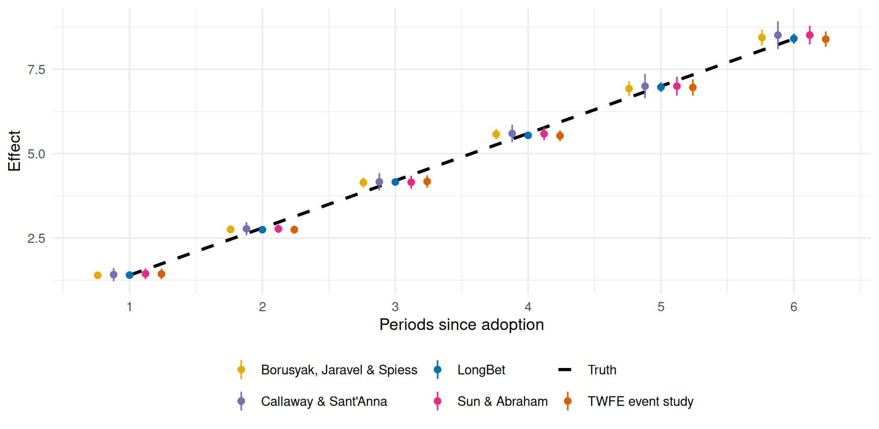
kable(score_curves(ad_curves, ad_truth), digits = 3,
caption = sprintf("Accuracy over the %d observed event times on one dataset. Containment counts are not coverage.", ad_max_s))| Estimator | RMSE | Mean error | Interval width | Contained truth |
|---|---|---|---|---|
| TWFE event study | 0.043 | -0.027 | 0.363 | 6 of 6 |
| Borusyak, Jaravel & Spiess | 0.047 | -0.029 | 0.331 | 6 of 6 |
| LongBet | 0.048 | -0.037 | 0.295 | 6 of 6 |
| Callaway & Sant’Anna | 0.049 | 0.010 | 0.397 | 6 of 6 |
| Sun & Abraham | 0.054 | 0.011 | 0.409 | 6 of 6 |
LongBet was not told that the world was additive, that the effect was homogeneous, or that the trajectory was linear, and it lands with the estimators built for exactly this case. That is the reassurance worth having before using a flexible model where the classical one cannot go: flexibility is not costing you anything here.
Why the canonical estimator needs repairing
The TWFE event study above is well behaved because it includes never-treated units and leads and lags. The single-coefficient TWFE regression that many teams still run is not. The Goodman-Bacon decomposition shows exactly why.
invisible(capture.output(ad_bacon <- bacon(y ~ treat, data = ad_long, id_var = "id", time_var = "time")))
ad_bacon %>% group_by(type) %>%
  summarise(Weight = sum(weight), `Weighted average estimate` = sum(estimate * weight) / sum(weight),
            .groups = "drop") %>%
  rename(`Comparison type` = type) %>%
kable(digits = 3, caption = "Goodman-Bacon decomposition of the static two-way fixed effects coefficient on this panel.")| Comparison type | Weight | Weighted average estimate |
|---|---|---|
| Earlier vs Later Treated | 0.259 | 2.604 |
| Later vs Earlier Treated | 0.270 | -1.171 |
| Treated vs Untreated | 0.470 | 3.504 |
The “later versus earlier treated” row is the forbidden comparison: it uses units that are already treated, and whose effects are still growing, as the control group. With a dynamic effect its two-by-two estimate is negative even though every unit’s effect is positive, and it carries a quarter of the total weight. That is the pathology the modern estimators remove, and it is why a single TWFE coefficient is not a safe default for a staggered rollout.
27.3 Where the Cell Estimators Cannot Go
Now a second panel with the same staggered design: 400 units, a trajectory that is concave rather than linear, and a size of the effect that varies smoothly with a covariate:
\[ \tau(x, S) = (1.5 + 0.9\,x_1)\,\log(1 + S). \]
Every estimator in this chapter can still recover the average. The difference appears below the average.
hd <- simulate_heterogeneous()
hd_long <- panel_long(hd)
hd_max_s <- max(hd$s[hd$z == 1])
hd_truth <- vapply(seq_len(hd_max_s), function(ss) mean(hd$tau[hd$s == ss]), numeric(1))
hd_run <- lb_artifact(
  "hetero_fit",
  lb_key("hetero", lb_budget(10), LB_MODEL, digest::digest(hd[c("y", "x", "z")])),
  export = "hd",
  builder = function() {
    f <- do.call(longbet::longbet, c(list(y = hd$y, x = hd$x, z = hd$z, t = hd$tg, random_seed = 303L),
                                     LB_MODEL, lb_budget(10)))
    p <- predict(f, x = hd$x, z = hd$z, t = hd$tg, random_seed = 1)
    list(att = get_att(p, alpha = 0.05),
         cell_draws = matrix(p$tauhats, nrow = length(hd$z))[as.vector(hd$z == 1), ],
         layout = chain_layout(f$model_params$num_chains, f$model_params$num_sweeps))
  })
hd_curves <- bind_rows(
  did_event_curves(hd_long, hd_max_s),
  tibble(s = seq_len(hd_max_s), estimate = hd_run$att$att[seq_len(hd_max_s)],
         lower = hd_run$att$intervals[1, seq_len(hd_max_s)],
         upper = hd_run$att$intervals[2, seq_len(hd_max_s)], estimator = "LongBet"))
hd_cell_draws <- hd_run$cell_draws
hd_cell_truth <- hd$tau[hd$z == 1]; hd_cell_s <- hd$s[hd$z == 1]
hd_cell_est <- rowMeans(hd_cell_draws)
kable(bind_rows(
  diagnose_draws(hd_run$att$att_full, hd_run$layout, "Average effect, every exposure")$summary,
  diagnose_draws(hd_cell_draws, hd_run$layout,
                 sprintf("Unit-period effects (%d cells)", nrow(hd_cell_draws)))$summary) %>%
    select(-ok), digits = 3,
caption = "Sampling checks for this panel, including every treated unit-period effect, the slowest-mixing quantities in the book.")| Quantity | R-hat (max) | Bulk ESS (min) | Tail ESS (min) | Passed |
|---|---|---|---|---|
| Average effect, every exposure | 1.001 | 7787.513 | 6824.679 | 6 of 6 |
| Unit-period effects (1194 cells) | 1.003 | 3936.208 | 3679.829 | 1194 of 1194 |
hd_curves %>% group_by(Estimator = estimator) %>%
  summarise(`Average-effect RMSE` = sqrt(mean((estimate - hd_truth)^2)),
            `Interval width` = mean(upper - lower), .groups = "drop") %>%
  arrange(`Average-effect RMSE`) %>%
kable(digits = 3, caption = "Every estimator recovers the average. The difference is what lies underneath it.")| Estimator | Average-effect RMSE | Interval width |
|---|---|---|
| TWFE event study | 0.067 | 0.361 |
| LongBet | 0.073 | 0.185 |
| Sun & Abraham | 0.075 | 0.402 |
| Callaway & Sant’Anna | 0.077 | 0.491 |
| Borusyak, Jaravel & Spiess | 0.086 | 0.467 |
cs_by_s <- hd_curves %>% filter(estimator == "Callaway & Sant'Anna") %>% arrange(s) %>% pull(estimate)
tibble(`Unit-period predictor` = c("LongBet posterior mean, per unit-period",
                                   "Callaway & Sant'Anna event-time average, imputed to every unit"),
       RMSE = c(sqrt(mean((hd_cell_est - hd_cell_truth)^2)),
                sqrt(mean((cs_by_s[hd_cell_s] - hd_cell_truth)^2))),
       `Correlation with truth` = c(cor(hd_cell_est, hd_cell_truth),
                                    cor(cs_by_s[hd_cell_s], hd_cell_truth)),
       `SD of the true effects` = sd(hd_cell_truth)) %>%
kable(digits = 3, caption = "Accuracy of unit-period effects. The aggregate estimator is not designed for this target; the row shows the cost of imputing its event-time average to every unit.")| Unit-period predictor | RMSE | Correlation with truth | SD of the true effects |
|---|---|---|---|
| LongBet posterior mean, per unit-period | 0.153 | 0.994 | 1.343 |
| Callaway & Sant’Anna event-time average, imputed to every unit | 1.197 | 0.453 | 1.343 |
bind_rows(tibble(truth = hd_cell_truth, estimate = hd_cell_est, which = "LongBet posterior mean"),
          tibble(truth = hd_cell_truth, estimate = cs_by_s[hd_cell_s],
                 which = "Callaway & Sant'Anna event-time average")) %>%
  ggplot(aes(truth, estimate)) +
  geom_abline(linetype = "dashed") +
  geom_point(alpha = 0.3, size = 0.8, colour = DID_PAL[["LongBet"]]) +
  facet_wrap(~ which) +
  labs(x = "True effect of the unit-period", y = "Estimate")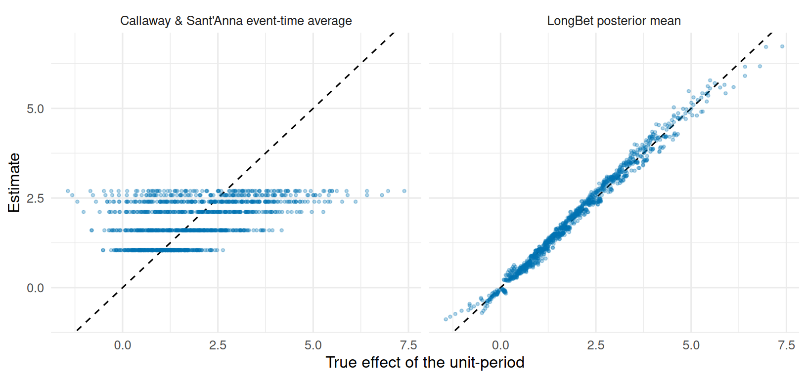
The right panel is not a criticism of the estimator; it is what a cohort-by-period average is. Every unit at a given exposure receives the same number, because that is the parameter being estimated.
27.4 What That Is Worth in a Decision
Make it a decision. Treating a unit-period is worth its effect minus a cost of 1.5, and each rule treats where its own estimate clears that cost. Every rule is scored on the true effects, including the rule of treating everyone, because a targeting rule that cannot beat “treat everyone” is not worth building.
value_of <- function(keep) sum(hd_cell_truth[keep] - 1.5)
tibble(Policy = c("Oracle (true effects)", "LongBet posterior mean",
                  "Callaway & Sant'Anna average by exposure", "Treat every unit-period"),
       `Unit-periods treated` = c(sum(hd_cell_truth > 1.5), sum(hd_cell_est > 1.5),
                                  sum(cs_by_s[hd_cell_s] > 1.5), length(hd_cell_truth)),
       `Net value` = c(value_of(hd_cell_truth > 1.5), value_of(hd_cell_est > 1.5),
                       value_of(cs_by_s[hd_cell_s] > 1.5), value_of(rep(TRUE, length(hd_cell_truth))))) %>%
  mutate(`Share of oracle value` = scales::percent(`Net value` / `Net value`[1], 0.1)) %>%
kable(digits = 1, caption = "Value of a targeting rule that treats unit-periods whose estimated effect exceeds the cost, scored on the true effects.")| Policy | Unit-periods treated | Net value | Share of oracle value |
|---|---|---|---|
| Oracle (true effects) | 664 | 873.8 | 100.0% |
| LongBet posterior mean | 638 | 871.3 | 99.7% |
| Callaway & Sant’Anna average by exposure | 907 | 598.3 | 68.5% |
| Treat every unit-period | 1194 | 463.5 | 53.0% |
An estimator that ranks exposures must treat every unit at an exposure or none of them. An estimator that ranks units can leave the unprofitable ones out. That gap is the case for a unit-level model in a targeting problem, and notice what it is not: it is not a gap in average accuracy, because the previous table showed the two agreeing on the average.
27.5 When Untreated Trends Diverge With the Covariates
Both panels so far had parallel trends: the covariates did nothing to the untreated path, so a difference against the not-yet-treated removed everything that was not the effect. That is the world the estimators above were built for, and it is not the only world. The simulation study of Wang et al. (2026) is built around the other one, and this section reproduces its design on a single pair of panels so the result can be read next to the paper’s tables.
Five hundred units over twelve periods. Five covariates: three standard normal, one binary, and one three-level factor, which the linear estimators receive as dummies. A unit’s untreated level depends on the covariates through the loading \(g(x_4) + x_1\,|x_3 - 1|\), with \(g(0) = 2\) and \(g(1) = -1\), a piece of the prognostic function of the BCF simulation design (Hahn et al. 2020): a step and a kink, nothing a linear adjustment can represent exactly. Adoption starts in period 7, and in every period from then on a unit that has not yet adopted does so with a probability that rises with its loading, so cohorts differ systematically in their untreated level. The effect factorizes as the model assumes, \(\nu(x)\,(1 - e^{-S/2})\), with \(\nu\) depending on two covariates that drive neither the level nor adoption, so that heterogeneity is not confounded with selection.
Two panels share everything, seed included, and differ in one line. Under parallel trends the units move together, driven by a common calendar factor. Under diverging trends each unit also drifts in proportion to its loading, so the units that adopt first are the ones whose untreated path was already climbing fastest, by an amount calibrated to be of the same order as the effect. Conditional on the covariates the trends are still parallel, because the drift is a function of recorded covariates and calendar time; unconditionally they are not.
pd <- list(parallel = simulate_paper_design(seed = 4, trend = "parallel"),
           diverging = simulate_paper_design(seed = 4, trend = "diverging"))
stopifnot(identical(pd$parallel$z, pd$diverging$z), identical(pd$parallel$tau, pd$diverging$tau))
pd_max_s <- max(pd$parallel$s)
pd_truth <- vapply(seq_len(pd_max_s), function(ss) mean(pd$parallel$tau[pd$parallel$s == ss]), numeric(1))
pd_budget <- list(parallel = lb_budget(2), diverging = lb_budget(10))   # unit-period effects are reported for the diverging panel
pd_runs <- lapply(pd, function(d) lb_artifact(
  paste0("paper_", d$trend),
  lb_key("paper_design", d$trend, pd_budget[[d$trend]], LB_MODEL, digest::digest(d[c("y", "x", "z")])),
  export = "pd_budget",
  builder = function() {
    f <- do.call(longbet::longbet, c(list(y = d$y, x = d$x, z = d$z, t = d$tg, random_seed = 404L),
                                     LB_MODEL, pd_budget[[d$trend]]))
    p <- predict(f, x = d$x, z = d$z, t = d$tg, random_seed = 1)
    list(att = get_att(p, alpha = 0.05),
         cell_draws = matrix(p$tauhats, nrow = length(d$z))[as.vector(d$z == 1), ],
         layout = chain_layout(f$model_params$num_chains, f$model_params$num_sweeps))
  }))
pd_long <- lapply(pd, panel_long)
tibble(Cohort = c(paste("Adopted in period", sort(unique(pd$parallel$adopt[is.finite(pd$parallel$adopt)]))), "Never adopted"),
       Units = c(as.vector(table(pd$parallel$adopt[is.finite(pd$parallel$adopt)])), sum(!is.finite(pd$parallel$adopt))),
       `Mean loading` = c(tapply(pd$parallel$loading, pd$parallel$adopt, mean)[as.character(sort(unique(pd$parallel$adopt[is.finite(pd$parallel$adopt)])))],
                          mean(pd$parallel$loading[!is.finite(pd$parallel$adopt)]))) %>%
kable(digits = 2, caption = "Adoption is confounded with the prognostic loading: earlier cohorts have higher untreated levels, and under diverging trends they also climb faster.")| Cohort | Units | Mean loading |
|---|---|---|
| Adopted in period 7 | 70 | 1.15 |
| Adopted in period 8 | 51 | 1.00 |
| Adopted in period 9 | 53 | 1.49 |
| Adopted in period 10 | 45 | 1.05 |
| Adopted in period 11 | 29 | 0.56 |
| Adopted in period 12 | 22 | 1.02 |
| Never adopted | 230 | -0.30 |
pd_curves <- imap_dfr(pd, function(d, nm) bind_rows(
  did_event_curves(pd_long[[nm]], pd_max_s, xformla = ~ x1 + x2 + x3 + x4 + x5, ife = TRUE),
  tibble(s = seq_len(pd_max_s), estimate = pd_runs[[nm]]$att$att[seq_len(pd_max_s)],
         lower = pd_runs[[nm]]$att$intervals[1, seq_len(pd_max_s)],
         upper = pd_runs[[nm]]$att$intervals[2, seq_len(pd_max_s)], estimator = "LongBet")) %>%
  mutate(panel = factor(if (nm == "parallel") "Parallel trends" else "Diverging trends",
                        levels = c("Parallel trends", "Diverging trends"))))
pd_cell_diag <- diagnose_draws(pd_runs$diverging$cell_draws, pd_runs$diverging$layout,
                               sprintf("Diverging trends: unit-period effects (%d cells)", nrow(pd_runs$diverging$cell_draws)))
pd_diag <- bind_rows(
  diagnose_draws(pd_runs$parallel$att$att_full, pd_runs$parallel$layout, "Parallel trends: average effect, every exposure")$summary,
  diagnose_draws(pd_runs$diverging$att$att_full, pd_runs$diverging$layout, "Diverging trends: average effect, every exposure")$summary,
  pd_cell_diag$summary)
kable(pd_diag %>% select(-ok), digits = 3,
caption = "Sampling checks for the two LongBet fits. The diverging panel, whose unit-period effects are reported below, runs five times longer chains than the parallel one, whose average effect is all that is used.")| Quantity | R-hat (max) | Bulk ESS (min) | Tail ESS (min) | Passed |
|---|---|---|---|---|
| Parallel trends: average effect, every exposure | 1.005 | 2188.085 | 7017.564 | 6 of 6 |
| Diverging trends: average effect, every exposure | 1.001 | 6840.717 | 7744.830 | 6 of 6 |
| Diverging trends: unit-period effects (1102 cells) | 1.052 | 102.438 | 431.057 | 707 of 1102 |
The average effects pass on both panels. The unit-period effects on the diverging panel do not all clear the gate at this budget: 707 of 1102 cells pass, and the largest R-hat is 1.05. That is the one place in these chapters where the sampler is visibly slow, and it is slow for a reason worth knowing. On this panel a unit’s own amplitude trades off against its covariate-linked trend, because the same covariates drive both, and the chains move along that direction one tree at a time; the paper’s own diagnostics single out the diverging heterogeneous design as the hardest of its six. The average effect is not affected, and the parallel panel’s cells mix as well as the previous section’s. Read the cell-level numbers on this panel as indicative, and treat the average-effect comparison, which is the point of the section, as settled.
ggplot(pd_curves, aes(s, estimate, colour = estimator)) +
  geom_line(data = tidyr::expand_grid(panel = levels(pd_curves$panel), tibble(s = seq_len(pd_max_s), estimate = pd_truth)) %>%
              mutate(estimator = "Truth", panel = factor(panel, levels = levels(pd_curves$panel))),
            linewidth = 1.1, linetype = "dashed") +
  geom_pointrange(aes(ymin = lower, ymax = upper), position = position_dodge(0.75), size = 0.22) +
  facet_wrap(~ panel) +
  scale_colour_manual(values = DID_PAL) +
  scale_x_continuous(breaks = seq_len(pd_max_s)) +
  labs(x = "Periods since adoption", y = "Effect", colour = NULL) +
  theme(legend.position = "bottom") + guides(colour = guide_legend(nrow = 3))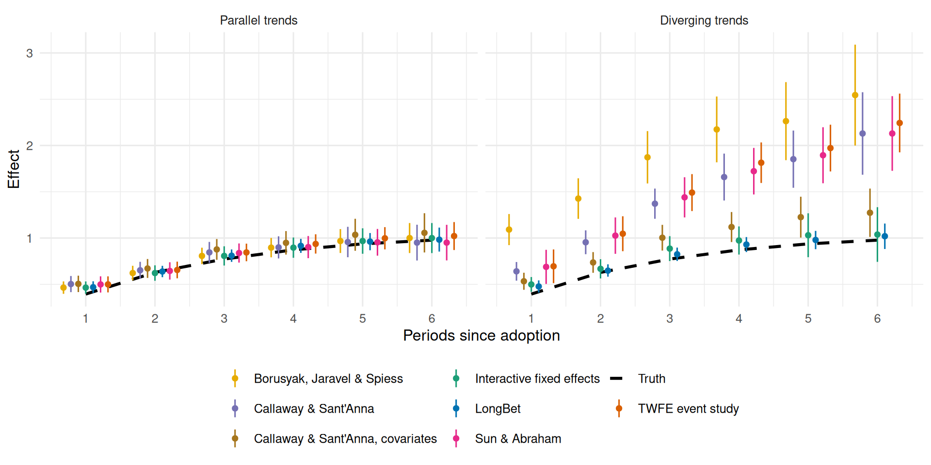
pd_curves %>% group_by(panel) %>% group_modify(~ score_curves(.x, pd_truth)) %>% ungroup() %>%
  rename(Panel = panel) %>%
kable(digits = 3, caption = sprintf("Accuracy over the %d observed event times, one dataset per panel. Containment counts are not coverage; the paper reports coverage over twelve replicates of each design.", pd_max_s))| Panel | Estimator | RMSE | Mean error | Interval width | Contained truth |
|---|---|---|---|---|---|
| Parallel trends | Borusyak, Jaravel & Spiess | 0.037 | 0.029 | 0.210 | 5 of 6 |
| Parallel trends | Interactive fixed effects | 0.037 | 0.029 | 0.221 | 5 of 6 |
| Parallel trends | LongBet | 0.040 | 0.032 | 0.164 | 5 of 6 |
| Parallel trends | Sun & Abraham | 0.054 | 0.034 | 0.247 | 5 of 6 |
| Parallel trends | Callaway & Sant’Anna | 0.057 | 0.037 | 0.256 | 5 of 6 |
| Parallel trends | TWFE event study | 0.067 | 0.062 | 0.216 | 5 of 6 |
| Parallel trends | Callaway & Sant’Anna, covariates | 0.088 | 0.085 | 0.272 | 5 of 6 |
| Diverging trends | LongBet | 0.053 | 0.049 | 0.174 | 5 of 6 |
| Diverging trends | Interactive fixed effects | 0.089 | 0.085 | 0.334 | 5 of 6 |
| Diverging trends | Callaway & Sant’Anna, covariates | 0.230 | 0.218 | 0.329 | 1 of 6 |
| Diverging trends | Callaway & Sant’Anna | 0.743 | 0.671 | 0.467 | 0 of 6 |
| Diverging trends | Sun & Abraham | 0.781 | 0.720 | 0.519 | 0 of 6 |
| Diverging trends | TWFE event study | 0.851 | 0.780 | 0.453 | 0 of 6 |
| Diverging trends | Borusyak, Jaravel & Spiess | 1.172 | 1.132 | 0.664 | 0 of 6 |
Read the table in the order the paper reports it. Where trends are parallel, every estimator recovers the curve, and LongBet’s intervals are among the narrowest for the reason the first chapter gave: with nothing for it to do, the horseshoe prior switches the covariate-trend half of the calendar-time block off. Where trends diverge, the estimators that condition on nothing but the rollout are misled by about as much as the effect they are estimating, by construction. Two survive it. Callaway and Sant’Anna with covariates conditions on them through a linear outcome regression and a logistic propensity score, and what remains of its error is the part of \(g(x_4) + x_1|x_3 - 1|\) that a linear adjustment cannot reach. Interactive fixed effects never sees the covariates: it fits a low-rank factor structure to the untreated panel, which this drift has exactly, at the price of estimating a loading for every unit from its own untreated periods. LongBet represents the conditional trend with a tree ensemble for the level, a free effect for every period, and smooth time profiles loaded on a dictionary of the covariates that contains the step in \(x_4\) exactly and a hinge in \(x_3\) that comes close to the kink. Across the twelve replicates of the paper’s study that combination halves the root mean squared error of interactive fixed effects on both diverging designs while keeping coverage near nominal; one panel cannot show coverage, but it can show the ordering.
div_curve <- function(label) pd_curves %>% filter(panel == "Diverging trends", estimator == label) %>% arrange(s) %>% pull(estimate)
pd_cell_truth <- pd$diverging$tau[pd$diverging$z == 1]; pd_cell_s <- pd$diverging$s[pd$diverging$z == 1]
pd_cell_est <- rowMeans(pd_runs$diverging$cell_draws)
pd_cell_lo <- apply(pd_runs$diverging$cell_draws, 1, quantile, 0.025)
pd_cell_hi <- apply(pd_runs$diverging$cell_draws, 1, quantile, 0.975)
broadcast <- function(label) div_curve(label)[pd_cell_s]
tibble(`Unit-period predictor` = c("LongBet posterior mean, per unit-period",
                                   "Callaway & Sant'Anna with covariates, imputed to every unit",
                                   "Interactive fixed effects, imputed to every unit"),
       RMSE = c(sqrt(mean((pd_cell_est - pd_cell_truth)^2)),
                sqrt(mean((broadcast("Callaway & Sant'Anna, covariates") - pd_cell_truth)^2)),
                sqrt(mean((broadcast("Interactive fixed effects") - pd_cell_truth)^2))),
       `Correlation with truth` = c(cor(pd_cell_est, pd_cell_truth),
                                    cor(broadcast("Callaway & Sant'Anna, covariates"), pd_cell_truth),
                                    cor(broadcast("Interactive fixed effects"), pd_cell_truth)),
       `Share of cells with the truth inside the 95% interval` =
         c(mean(pd_cell_truth >= pd_cell_lo & pd_cell_truth <= pd_cell_hi), NA, NA)) %>%
kable(digits = 3, caption = sprintf("Unit-period effects on the diverging-trends panel, %d treated cells. Only LongBet produces a cell-level interval; the comparison rows broadcast an event-time average, as the paper's unit-level table does.", length(pd_cell_truth)))| Unit-period predictor | RMSE | Correlation with truth | Share of cells with the truth inside the 95% interval |
|---|---|---|---|
| LongBet posterior mean, per unit-period | 0.158 | 0.905 | 0.883 |
| Callaway & Sant’Anna with covariates, imputed to every unit | 0.353 | 0.569 | NA |
| Interactive fixed effects, imputed to every unit | 0.301 | 0.570 | NA |
The same assumption, two differences
It would be easy to read this section as LongBet assuming less than the difference-in-differences estimators. It does not. Its identifying assumption is that once the covariates and a unit’s persistent level are known, the adoption date carries no further information about the untreated path; together with the additive level inside the model, that implies parallel trends conditional on the covariates, so the model belongs to the same family as the covariate-adjusted estimators rather than being an alternative to it. Two things differ, and neither is a weaker assumption.
The first is what the conditional trend is allowed to be. The doubly robust implementation of Callaway and Sant’Anna (2021) represents it with a linear outcome regression and a logistic propensity score in the supplied covariates. LongBet represents it with a tree ensemble for the level, a complete basis for the common movement of every period, and smooth time profiles loaded on a nonlinear feature map of the covariates, under a prior that keeps the unused terms at zero. The diverging panel above satisfies conditional parallel trends with a conditional trend that is nonlinear in the covariates, and that is exactly the case that separates the two.
The second is what the model does with the unit’s level once it has it. Differencing removes a level correlated with adoption timing exactly, whatever that correlation is. LongBet estimates the level and shrinks it toward an exchangeable prior, and the fourth chapter puts a number on what that costs when a unit has only one or two untreated periods. In exchange, the same fit delivers an effect that varies across units rather than across cohorts, a trajectory pooled across cohorts and projectable past the panel, and intervals that are narrower when the additional structure is right.
27.6 How to Choose
- Use the econometric estimators when the question is the average effect of a staggered rollout, when unconditional parallel trends is plausible or the covariates enter the trend linearly, when the panel is large and the model should be as transparent as possible, or when a reviewer needs an estimator with published guarantees and pre-trend diagnostics. They are fast, they are well understood, and on their home turf nothing beats them.
- Use LongBet as well when the decision needs a number per unit rather than per period, when the untreated paths of different kinds of units plausibly diverge in ways a linear adjustment will not capture, when you want the trajectory projected past the end of the study, when several outcomes must be screened together, or when the deliverable is a probability that a specific unit clears a specific bar.
- Run both, and report both. They estimate the same average from the same data under the same family of assumptions, so agreement is a real check on the model and a disagreement is information: it says that the linear conditional trend and the flexible one disagree about where the untreated cohorts were headed, which is a substantive question about the panel rather than a modelling detail. The LongBet chapters keep a design-based estimate alongside the model wherever the design provides one, for exactly this reason.
TipLearn more
- Goodman-Bacon (2021) on the decomposition of the two-way fixed effects estimator.
- Callaway and Sant’Anna (2021) on group-time average treatment effects, with and without covariates.
- Sun and Abraham (2021) on interaction-weighted event studies.
- Borusyak et al. (2024) on imputation estimators.
- Xu (2017) and Liu et al. (2024) on interactive fixed effects and counterfactual estimators.
- Roth et al. (2023) for a survey of what is now standard practice.
- Wang et al. (2026) for the full simulation study this section reproduces one panel of.